Summary: The tm and lsa packages provide you a way of manipulating your text data into a term-document matrix and create new, numeric features.  The ngram package lets you find frequent word patterns (e.g. “The cow” is a bi-gram or 2-gram; “The cow said” is a tri-gram or 3-gram).  Lastly, for a quick visualization (though not that informative), you can use the wordcloud package.

I’ve been working with some (relatively) large text analyses and I’ve noticed that R has quite a few packages (see the NLP View on CRAN) but there aren’t a lot of resources exploring all of these text mining tools.  To follow along you can download the code.

TM: The Text Mining Package

This is the main workhorse, in my opinion, of R’s natural language processing tools.  It includes…

• A way to covert files, directories, data frames, and vectors into a Corpus.
• Stemming. tm_map(corpus, stemDocument, "english")
• Removing numbers, punctuation, and multiple spaces tm_map(corpus, removeNumbers); tm_map(corpus, removePunctuation); tm_map(corpus, stripWhitespace);
• Removing stopwords tm_map(corpus,removeWords,stopwords("english"))

For example, let’s say you happened to have a bunch of text across many documents.

You can load that data into a “Corpus” which will let you manipulate it with tm_map. I’m using a variable called story_string which has each document as an element of a character vector.

corp <- VCorpus(VectorSource(story_string))
corp <- tm_map(corp,PlainTextDocument)
corp <- tm_map(corp,content_transformer(tolower))
corp <- tm_map(corp,removePunctuation)
corp <- tm_map(corp,removeWords,stopwords("en"))
tdm <- TermDocumentMatrix(corp)

Now with a Term Document Matrix (where each row is a term and each document is a column) you can do some basic analysis with the specialized {tm} functions.

If you want to see what are the most common terms, you can call findFreqTerms(TermDocMatrix,lowfreq=X, highFreq=Inf). This will return an alphabetized list of the top words. It’s not exactly useful so we can do some simple R functions to get the words and the total counts.

#Finding Frequent Terms
findFreqTerms(tdm,lowfreq = 169)

#Getting count of words
termcount <-apply(tdm,1,sum)
head(termcount[order(termcount,decreasing = T)],20)

The second code snippet will return the list of words in order of descending frequency rather than alphabetically.

You can also find associations using the findAssocs(corpus, c("term1",...,"termN"), c(strength1,...,strengthN)) function. You can select multiple terms and varying levels of association. However, as it turns out, the function is just looking at correlation between terms. You could get the relationship (i.e. correlation) between two terms by converting the Term Doc Matrix to an actual matrix and then calculating the correlation between the two columns.

#Convert term Doc Matrix and Transpose it for ease.
dtm_mat <- t(as.matrix(tdm))

#Calculate the correlation between
cor(dtm_mat[,colnames(dtm_mat)=="term1"],
    dtm_mat[,colnames(dtm_mat)=="term2"])

I’m surprised the {tm} package doesn’t provide a co-occurrence association function. It might be worth experimenting with the {arules} package to find association rules.

Wordcloud: Create Simple Word Clouds in R

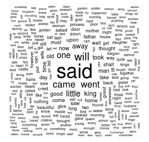
I think word clouds are an interesting but not always useful.  Regardless, there is a {wordcloud} package available in R with a very simple syntax.

All you need is a vector of words and a vector of frequencies.  Earlier in this example, we calculated a termcount variable but summing the rows of a term document matrix.

wordcloud(names(termcount),termcount,
          min.freq=10,random.order=FALSE)

It’s as simple as that! You can also add in things like colors. While not great for analysis purposes, it does produce a nice image!

NGRAM: Find Common Patterns

The {ngram} package is a simple tool that contains a way to identify different “N-Grams“.  I really like the author’s of the package.  The documentation has a bit of sass and I respect that.

An N-Gram is a pattern of N words that appear in a corpus.  It’s very common to see bi-grams (two words) or tri-grams (three words).  The {ngram} package relies on the ngram function.

#Needs a character vector or block of text
ng <- ngram(character_variable,n=2)
print(ng,full=TRUE)

This will print a list of bi-grams that are found. Useful if you have a few of them. Too much data if there are a lot of them.

I think there’s some potential in here for mapping patterns as in word trees.  But that’s clearly something for later.

My favorite part of this package (and the reason why I chose it over {tau}) is the babble function babble(ng,n)!  With an ngram, you can essentially produce new text by assessing what’s the next most likely term.

Here’s the passage I created by analyzing 61 stories from the Brother’s Grimm.

“…you come to the village, the son sat down on the side of the princess, the horse, and the bank was so big that the two men were his brothers, who had turned robbers; so he took up the golden cage, and the three golden apples that had been lost were lying close by it stands a beautiful garden, and in a moment the fox said; they carried off the bird, and his country too. Time passed on; and as the eldest son to watch; but about twelve o’clock at night the princess going to the shabby cage and put…”

It’s actually passable!

The drawbacks to the {ngram} package is that it doesn’t work with the {tm} package’s Corpus.  It would be very nice to be able to use this same tm_map functions to clean up the text.

LSA: Latent Semantic Analysis

So far, we haven’t really done any analysis of our text.  tm is great for massaging your data.  wordcloud produces a nice visual.  ngram provides you some cool information on patterns of words.

Latent Semantic Analysis uncovers latent features, or topics, within your documents.

There’s a bit of redundancy for utility functions in LSA as there are are in tm.

• Removing stopwords, stemming, min/max word lengths using the textmatrix function.
• Weighting a text matrix including tf-idf lw_logtf(matrix) * gw_idf(matrix).
• A unique one, as far as I can tell, is the lw_bintf which checks each cell if its value is greater than zero.  Better than having to write your own function for it.

After creating a textmatrix, we can run the LSA function (and by default it searches for an appropriate number of topics).

txt_mat<- as.textmatrix(as.matrix(tdm))

lsa_model <- lsa(txt_mat)

dim(lsa_model$tk) #Terms x New LSA Space
dim(lsa_model$dk) #Documents x New LSA Space
length(lsa_model$sk) #Singular Values

You can do some basic analysis of the terms or documents.  This is where you would apply other data mining efforts and inference of the new “feature space”.  For example, you might create a dendrogram to see if there are any obvious clusters of documents.

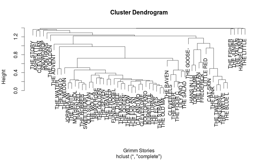
This is where text mining begins to look more like “regular” data mining.  As you engineer new features (as you create a “latent semantic space”), you now have quantitative variables you can work with in algorithms like regression, support vector machines, and neural networks.

Bottom Line:  The TM package is your main workhorse of text mining in R.  If you want to engineer new features, try LSA or its similar packages (LDA, topicmodels).