This tutorial covers the basics of working with the rpart library and some of the advanced parameters to help with pre-pruning a decision tree.

If you’re not already familiar with the concepts of a decision tree, please check out this explanation of decision tree concepts to get yourself up to speed. Fortunately, R’s rpart library is a clear interpretation of the classic CART book.

Libraries Needed: rpart, rpart.plot

Data Needed: http://archive.ics.uci.edu/ml/datasets/Bank+Marketing (bank.Zip)

rpart(y~., data, parms=list(split=c("information","gini")),
      cp = 0.01, minsplit=20, minbucket=7, maxdepth=30)

Data Understanding

When dealing with a classification problem, you’re looking for opportunities to exploit a pattern in the data. It’s also very important to note that, for decision trees, you’re looking for linear patterns.

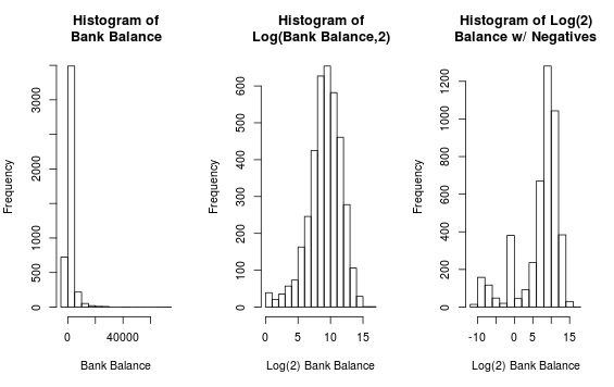
The bank balance is also something to look into.

Modeling

We’ll explore a few different ways of using rpart and we’ll explore the different parameters you can apply.

Basic Tree With Default Parameters

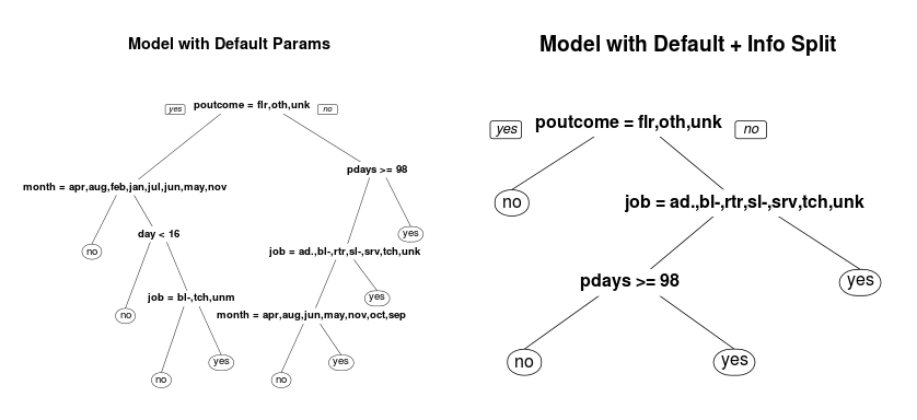
default.model <- rpart(y~., data = train)
info.model <- rpart(y~., data = train, parms=list(split="information"))

• The default splitting method for classification is “gini”.
• To define the split criteria, you use parms=list(split="...")

You can see that just changing the split criteria has already created a very different looking tree. Explaining the differences between gini index and information gain is beyond this short tutorial. But I have written a quick intro to the differences between gini index and information gain elsewhere.

Choosing between the gini index and information gain is an analysis all in itself and will take some experimentation.

Minsplit, Minbucket, Maxdepth

overfit.model <- rpart(y~., data = train, 
                       maxdepth= 5, minsplit=2, 
                       minbucket = 1)

One of the benefits of decision tree training is that you can stop training based on several thresholds. For example, a hypothetical decision tree splits the data into two nodes of 45 and 5. Probably, 5 is too small of a number (most likely overfitting the data) to have as a terminal node. Wouldn’t it be nice to have a way to stop the algorithm when it encounters this situation?

The option minbucket provides the smallest number of observations that are allowed in a terminal node. If a split decision breaks up the data into a node with less than the minbucket, it won’t accept it.

The minsplit parameter is the smallest number of observations in the parent node that could be split further. The default is 20. If you have less than 20 records in a parent node, it is labeled as a terminal node.

Finally, the maxdepth parameter prevents the tree from growing past a certain depth / height. In the example code, I arbitrarily set it to 5. The default is 30 (and anything beyond that, per the help docs, may cause bad results on 32 bit machines).

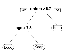
You can use the maxdepth option to create single-rule trees. These are examples of the one rule method for classification (which often has very good performance).

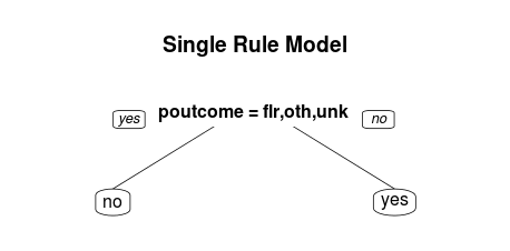
one.rule.model <- rpart(y~., data=train, maxdepth = 1)
rpart.plot(one.rule.model, main="Single Rule Model")

All of these options are ways preventing a model from overfitting via pre-pruning. However, there’s one more parameter you may need to adjust…

cp: Complexity Parameter

The complexity parameter (cp) in rpart is the minimum improvement in the model needed at each node. It’s based on the cost complexity of the model defined as…

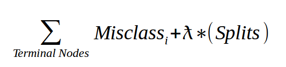
• For the given tree, add up the misclassification at every terminal node.
• Then multiply the number of splits time a penalty term (lambda) and add it to the total misclassification.
• The lambda is determined through cross-validation and not reported in R.
• The cp we see using printcp() is the scaled version of lambda over the misclassifcation rate of the overall data.

The cp value is a stopping parameter. It helps speed up the search for splits because it can identify splits that don’t meet this criteria and prune them before going too far.

If you take the approach of building really deep trees, the default value of 0.01 might be too restrictive.

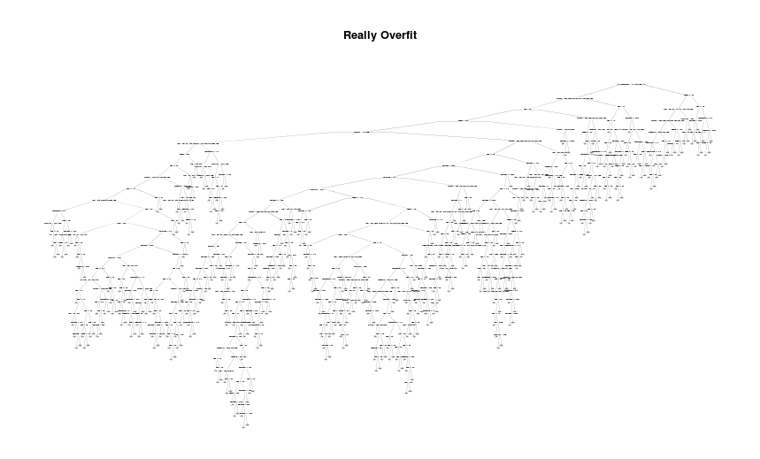
super.overfit.model <- rpart(y~., data = train, minsplit=2,
                       minbucket = 1, cp = 0.0001)
rpart.plot(super.overfit.model, main = "Really Overfit")

Using a Loss Matrix

The final option we’ll discuss is using the loss matrix from the parms list. Imagine you’re running a marketing campaign that offers some incredible discount for high-value customers you expect to leave.

Getting this prediction is very important. Not only for the obvious reason of wanting to keep these high-value customers but also due to the fact that your prediction has a real cost to it.

If you mistake a normal customer for one that is about to leave, your discount is throwing away money. So rpart offers a loss matrix.

cost.driven.model <- rpart(y~.,data=train, 
                           parms=list(
                             loss=matrix(c(0,1,5,0), 
                                         byrow=TRUE, 
                                         nrow=2))
                           )
#The Matrix looks like...
#     [,1] [,2]
#[1,]    0    1
#[2,]    5    0

The loss matrix is structured with actuals on the rows and predictions on the columns. When dealing with multiple classes, your matrix will look slightly different. Here’s what the confusion matrix looks like for my example.

            Predicted
Actual         Class1  Class2
        Class1     TP      FN
        Class2     FP      TN
**Assuming Class1 is the positive class.

So for this given situation, it’s 5 times worse to generate a false positive than a false negative. This will have the effect of making Class1 predicted less frequently. This makes sense since your loss matrix says “Watch out for being wrong on Class1!! I’d rather you said Class2 if you’re not really certain it’s Class1…”

A few notes on working with the Loss Matrix in R:

• The order of the loss matrix depends on the order of your factor variable in R.
• If you have multiple classes, think of it in terms of rows. “How much does it cost us if this real class is marked as something else”.
• The diagonal should always be zero and the non-diagonal values should be greater than zero.
• For example, for a four class problem, if you want to make Class2 the “positive” variable, you should mark all non-zero entries for that row with some cost.

    [,1] [,2] [,3] [,4]
[1,]    0    1    1    1
[2,]    5    0    5    5
[3,]    1    1    0    1
[4,]    1    1    1    0

Interpreting RPart Output

So you’ve built a few model by now. Let’s get analyzing with a few key functions.

• rpart.plot from the rpart.plot package prints very nice decision trees.
• print(rpart_model) Produces a simple summary of your model at each split. Shows…
  • Split criteria
  • # rows in this node
  • # Misclassified
  • Predicted Class
  • % of rows in predicted class for this node.
• printcp(rpart_model) the cp table showing the improvement in cost complexity at each node
• summary(rpart_model) the most descriptive output, providing…
  • CP Table
  • Variable Importance
  • Description of the Node and Split (including # going left or right and even surrogate splits.
  • Can be very verbose, so print with caution
• predict(rpart_model, newdata, method="class") lets you apply the model to new data. Using the “class” method, it will return the most likely class label.

There’s still more to the rpart function! There are prior probabilities and weighting observations. There are variable costs (and not just classification costs). There are poisson and anova splitting methods. However, this tutorial has covered the basics and some of the advanced parameters.

Keep experimenting and pushing your decision tree knowledge!