Summary: Logistic regression produces coefficients that are the log odds. Take e raised to the log odds to get the coefficients in odds. Odds have an exponential growth rather than a linear growth for every one unit increase. A two unit increase in x results in a squared increase from the odds coefficient. To get a probability you put the predicted odds through the logistic function of X / (1 + X).

Logistic Regression is related to Linear Regression by its use of the linear equation inside the logistic function.

It’s tempting to interpret them the same way but every stats 102 class will tell that you can’t! I took it upon myself to better understand what exactly is happening in logistic regression and how to better interpret the coefficients. Using the iris data set and a quick R program, I will show the differences between log odds, odds, and probability. Full disclosure, I had to open up three textbooks, and at least 12 webpages to gather enough understanding. Links to my favorite pages at the bottom.

Setting up the Data

data(iris)

# Turn this into a binary setosa vs not setosa problem
iris$Species <- as.factor(as.numeric(iris$Species == 'setosa'))

# Create a logistic regression model
model <- glm(Species~Sepal.Width, data=iris, family='binomial')

# Create a sequence of data in a data.frame to use for predictions
test_data <- data.frame(Sepal.Width = seq(0.1, 5.5, by=0.1))

First step we need to get the iris data set loaded and transform the Species variable to be binary. We could do multinomial logistic regression but that makes it more completed and doesn’t help with explaining the difference between log odds, odds, and probabilities too much.

To create a logistic regression model in R you use the glm function and the binomial family. Lastly, a sequence of numbers in a data.frame is created. This sequence will be all the values that the model will predict on to see the full spectrum of what is happening behind log odds, odds, and probabilities.

Log Odds

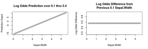
• The logistic regression coefficients are log odds.
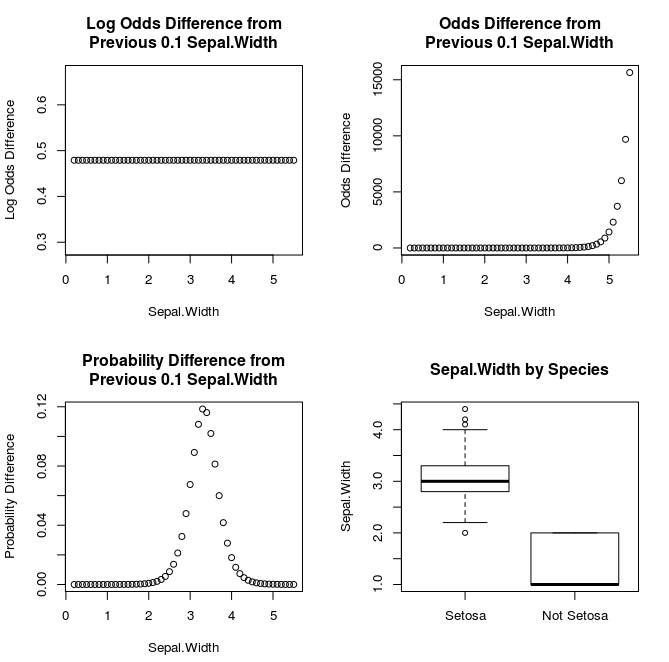
• Just like in regression, as you increase the input variable by one unit, the log odds increases by one unit
• The difference between each data point (right plot) is the same as the coefficient.

# Predict Log Odds Value
log_odds_pred <-predict(model, newdata=test_data)
diff(log_odds_pred)

model$coefficients #in Log Odds

The predict function simply takes the values of our test_data data.frame and inserts them into the learned logistic regression formula. You can see the model coefficients by using model$coefficients.

If you are comfortable with log odds, go no further! If you can explain what a one unit increase in the log odds means to your manager, you’re all set here. For those who still need some assistance read on.

Odds

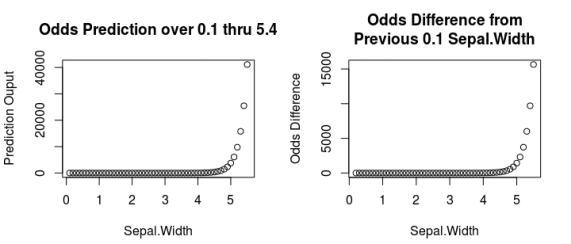
• The ‘odds’ are e (euler’s number) raised to log odds value.
• If you remember college algebra: e^(log(x)) = x
• From the plots above, you can see that as Sepal.Width increases, so does the odds of it being Setosa.
• The difference plot doesn’t show a different pattern since it’s a fast growing exponential trend.

odds_pred <- exp(log_odds_pred)
diff(odds_pred)

exp(model$coefficients[2]) #120.2574 
odds_pred[11]/odds_pred[1] #120.2574 

In this example, the odds are interpreted as # of setosa appearing at this sepal width for every one non-setosa. Logistic regression estimates the odds / the log odds since it does not take on a bounded value (e.g. between zero and one). It’s hard to tell in the example but if you’re following along, you’ll see that at 3.3 sepal width, the odds become greater than one.

• Odds less than 1 mean there’s a negative relationship between the independent and dependent variables.(Pr < 0.5)
• Odds equal to 1 mean there’s no relationship (it’s 50/50). (Pr = 0.5)
• Odds greater than 1 mean there’s a direct positive relationship. (Pr > 0.5)

To better understand the interpretation of odds on a continuous variable, we can look at the the exponentiated sepal width coefficient and the quotient of the 11th (1.1) and the 1st (0.1) odds prediction. They’re the same. But why?

For a continuous variable, for every one unit increase in the X variable, there is a relative and exponential effect.

• Odds are relative, so you need a baseline to compare against.
• If you knew the odds at sepal width = 2 were 0.00215565 and the exponentiated coefficient was 120.2574…
  • You can say at sepal width = 3, the odds are 122.2574 times more likely to be setosa than at sepal.width = 2.
  • The odds at sepal width 3 are 0.2592329 which is equal to 0.00215565 * 120.2574.
  • The odds at sepal width 4 are 120.2574 times greater than at width 3 but are 120.2574 squared (14461.85) times greater than width 2.
  • The equation for this might look like: Base_Odds(i) * Odds_Coefficient^(k-i) | in the example above, k would be 4 and i would be 2.
• With the example above, you can see that every unit increase isn’t a simple multiplication like linear regression.
• Instead, it’s an exponential increase relative to some baseline unit.

So if you are going to interpret the coefficients, you’ll have to say a one unit increase in sepal width is a ~4.79 increase in the log odds or a ~120.26 increase in the odds of being setosa. Personally, numbers this large value makes it hard to explain. Odds that are less than 10 would be more palatable – wrap your head around 4x larger vs 48x larger; the latter is hard to fathom. In this case, I might use a common value as an example and a one unit increase and the plots above to illustrate the interpretation.

Perhaps the best area to report and still interpret is the probability.

Probability

• Probability is calculated by entering the odds into the logistic or “logit” function
• The formula is… x / (1 + x) where x is a given odd.
• In Generalized Linear Model terms, this is the canonical link function for a binomial distribution.
• Notice how the probabilities follow a sigmoid / logistic curve (left plot) and are bound between zero and one.
• Based on the differences, you can see how it quickly increases as it approaches the center of the logistic curve (~3.3).
• Then the growth of the probabilities decreases since it’s bounded to a maximum of one.

probs <- odds_pred / (1+odds_pred)
# or using the predict function, the model, and the test data
resp_pred <-predict(model, newdata=test_data, type='response')

It’s important to note that the predict function will do all of this work to get down to probabilities if you use the type='response' parameter and argument. The predict function knows to use the logit link function since we declared the family was binomial and logit is the default link. You can verify that with model$family. Using predict is much more convenient than doing all the math yourself.

There we have it! We’ve gone from log odds coefficients, to odds (using euler’s number), to probabilities (using the logistic / logit / link function). Hopefully now you can remember that when interpreting the logistic regression coefficients you should…

• Take e raised to the log odds coefficient to get the odds exp(model$coefficients)
• Interpret the odds as an exponential trend.
• Say sepal width = 2 has 120 times higher odds to be setosa than sepal width = 1.
• Bring some example probabilities. For example:
  • Sepal width = 1 has a less than 0.00% probability of being setosa.
  • sepal width 3.3 has a 52% probability of being setosa.

Further Reading and Full Code

For those interested in additional interpretations, here are some of the most useful pages I found:

• Why use Odds Ratios? from the Analysis Factor blog
• Calculating odds and probabilities from a Clinical Trial knowledge base
• Converting Logit to Probability by Sebastian Sauer of FOM University
• Interpreting Binary Logistic Regression from Statistics Solutions

If you’re interested in recreating these results, here’s the full code including plots.

# Setup ####
data(iris)

iris$Species <- as.factor(as.numeric(iris$Species == 'setosa'))

# Create a logistic regression model
model <- glm(Species~Sepal.Width, data=iris, family='binomial')

# Create a sequence of data in a data.frame to use for predictions
test_data <- data.frame(Sepal.Width = seq(0.1, 5.5, by=0.1))

# Log Odds ####
# Predict Log Odds Value
log_odds_pred <-predict(model, newdata=test_data)
diff(log_odds_pred)

model$coefficients #in Log Odds

par(mfrow=c(1,2))
plot(x=test_data$Sepal.Width, y=log_odds_pred,
     xlab="Sepal.Width",ylab='Prediction Ouput',
     main='Log Odds Prediction over 0.1 thru 5.4')
plot(x=test_data[-1,], y=round(diff(log_odds_pred), 7),
     xlab='Sepal.Width', ylab='Log Odds Difference',
     main='Log Odds Difference from\nPrevious 0.1 Sepal.Width')

# Odds ####
odds_pred <- exp(log_odds_pred)
diff(odds_pred)

exp(model$coefficients[2]) #120.2574 
odds_pred[11]/odds_pred[1] #120.2574 

par(mfrow=c(1,2))
plot(x=test_data$Sepal.Width, y=odds_pred,
     xlab="Sepal.Width",ylab='Prediction Ouput',
     main='Odds Prediction over 0.1 thru 5.4')
plot(x=test_data[-1,],y=diff(odds_pred),
     xlab='Sepal.Width',ylab='Odds Difference',
     main='Odds Difference from\nPrevious 0.1 Sepal.Width')

# Probabilities ####
prob <- odds_pred / (1+odds_pred)
# or using the predict function, the model, and the test data
resp_pred <-predict(model, newdata=test_data, type='response')

par(mfrow=c(1,2))
plot(x=test_data$Sepal.Width, y=prob,
     xlab="Sepal.Width",ylab='Probability',
     main='Probability Prediction over 0.1 thru 5.4')
plot(x=test_data[-1,], y=diff(prob),
     xlab='Sepal.Width',ylab='Probability Difference',
     main='Probability Difference from\nPrevious 0.1 Sepal.Width')

# Head Plot ####
par(mfrow=c(2,2))
plot(x=test_data[-1,], y=round(diff(log_odds_pred), 7),
  xlab='Sepal.Width', ylab='Log Odds Difference',
  main='Log Odds Difference from\nPrevious 0.1 Sepal.Width')
plot(x=test_data[-1,],y=diff(odds_pred),
     xlab='Sepal.Width',ylab='Odds Difference',
     main='Odds Difference from\nPrevious 0.1 Sepal.Width')
plot(x=test_data[-1,], y=diff(resp_pred),
     xlab='Sepal.Width',ylab='Probability Difference',
     main='Probability Difference from\nPrevious 0.1 Sepal.Width')
boxplot(x=iris$Sepal.Width, iris$Species,
        names = c('Setosa','Not Setosa'),ylab='Sepal.Width',
        main='Sepal.Width by Species')