In a nutshell, the Central Limit Theorem states that the larger the sample size, the more confident we can be in our estimate of the true mean.

If you were to take repeated samples from a population (e.g. send out surveys to a random set of your customers multiple times, asking the same questions), average each sample and then use those averages to create a histogram, you could use those results to estimate where the true mean lies.

B2B Example: Let’s say you wanted to better understand the number of employees for each of your customers.  We’ll do this two ways: Working through the central limit theorem (hard way) and then applying the central limit theorem (easy way).

So let’s say you have some 5,000 customers that are businesses and have an unknown number of employees working at each of those businesses.  Someone asks “Who are we really selling to?  Are these big businesses or are they mom and pop stores?”

The question becomes, what is the average number of employees for your customers.

The Hard Way: To get a really good estimate, you could randomly sample you clients multiple times and then treat average each sample and use all averages as your distribution of the true (population) mean.

So let’s take 20 sample of 10 customers:

Sample 1:  75  89 100  73 112 114 110 108  94 124 | Avg = 99.9

Sample 2: 111  69 106  63 121 117 108  90  92 101 | Avg =  97.8

….

Sample 20: 93  51 111  94 121 108  55 100  83 103 | Avg = 91.9

If we plot the average of those 20 samples in a histogram, it looks close enough to normal to use the standard normal table to estimate the mean at 95% confidence.

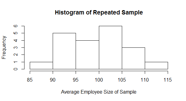
• Mean of samples = 99.49
• Standard Deviation of samples = 6.71

The 95% confidence interval around the mean is 88.45 – 110.53 (Mean +/- 1.64*(Standard Deviation).

The Easier Way (Applying the Central Limit Theorem):

So let’s say you didn’t want to take 20 samples of 10 customers each.  When your data is not heavily skewed, you can use a concept called the standard error.

Standard Error = sample standard deviation / square root of the sample size.

If we think about the idea of repeated samples, you’ll recognize that more data is more powerful.  The standard error uses the sample size as a way of controlling the impact of the sample standard deviation.

The rule of thumb is that you must have at least 30 observations to have enough data to apply the central limit theorem.

• Take a sample of 30 data points.
• Find the average and standard deviation of that sample.
• Then, calculate a 95% confidence interval with the standard error rather than the standard deviation.

Walk-Through:

[1] 99.9 97.8 101.8 108.1 101.8 96.0 113.4 102.3 98.9 91.2 91.0
[12] 100.5 107.5 102.1 88.0 107.4 94.3 103.3 92.6 91.9

Average = 99.23333

Standard Deviation = 6.710785

Standard Error = 6.710785 / Square-Root(30) = 2.73659

95% Confidence Interval of customer employee size using one sample and standard error = 94.73 – 103.74

The slightly improved interval is probably just a coincidence but it proves the point that this method works.

Warning:  There’s only one reason I can think of to estimate the mean the hard way, that’s to control for bias.  Taking dedicated samples for each segment of your customer file might be more representative if your data is skewed than taking just a random sample.

Bottom-Line: More data = tighter confidence interval when using the standard error to estimate your mean statistic.