Summary: The kmeans() function in R requires, at a minimum, numeric data and a number of centers (or clusters). The cluster centers are pulled out by using $centers. The cluster assignments are pulled by using $cluster. You can evaluate the clusters by looking at $totss and $betweenss.
Tutorial Time: 30 Minutes
R comes with a default K Means function, kmeans(). It only requires two inputs: a matrix or data frame of all numeric values and a number of centers (i.e. your number of clusters or the K of k means).
kmeans(x, centers, iter.max = 10, nstart = 1,
 algorithm = c("Hartigan-Wong", "Lloyd", "Forgy",
 "MacQueen"), trace=FALSE)
- X is your data frame or matrix. All values must be numeric.
- If you have an ID field make sure you drop it or it will be included as part of the centroids.
- Centers is the K of K Means. centers = 5 would results in 5 clusters being created.
- You have to determine the appropriate number for K.
- iter.max is the number of times the algorithm will repeat the cluster assignment and moving of centroids.
- nstart is the number of times the initial starting points are re-sampled.
- In the code, it looks for the initial starting points that have the lowest within sum of squares (withinss).
- That means it tries “nstart” samples, does the cluster assignment for each data point “nstart” times, and picks the centers that have the lowest distance from the data points to the centroids.
- trace gives a verbose output showing the progress of the algorithm.
K Means Algorithms in R
The out-of-the-box K Means implementation in R offers three algorithms (Lloyd and Forgy are the same algorithm just named differently).
The default is the Hartigan-Wong algorithm which is often the fastest. This StackOverflow answer is the closest I can find to showing some of the differences between the algorithms.
Research Paper References:
Forgey, E. (1965). “Cluster Analysis of Multivariate Data:
Efficiency vs. Interpretability of Classification”. In: Biometrics.

Lloyd, S. (1982). “Least Squares Quantization in PCM”.
In: IEEE Trans. Information Theory.

Hartigan, J. A. and M. A. Wong (1979). “Algorithm AS
136: A k-means clustering algorithm”. In: Applied Statistics
28.1, pp. 100–108.

MacQueen, J. B. (1967). “Some Methods for classification
and Analysis of Multivariate Observations”. In: Berkeley
Symposium on Mathematical Statistics and Probability
kmeans() R Example
Let’s take an example of clustering customers from a wholesale customer database. You can download the data I’m using from the Berkley UCI Machine Learning Repository here.
Let’s start off by reading in the data (Note: You may have to use setwd() to change your directory to wherever you’re storing your data). After reading in the data, let’s just get a quick summary.
data <-read.csv("Wholesale customers data.csv",header=T)
summary(data)
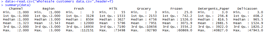
There’s obviously a big difference for the top customers in each category (e.g. Fresh goes from a min of 3 to a max of 112,151). Normalizing / scaling the data won’t necessarily remove those outliers. Doing a log transformation might help. We could also remove those customers completely. From a business perspective, you don’t really need a clustering algorithm to identify what your top customers are buying. You usually need clustering and segmentation for your middle 50%.
With that being said, let’s try removing the top 5 customers from each category. We’ll use a custom function and create a new data set called data.rm.top
top.n.custs <- function (data,cols,n=5) { #Requires some data frame and the top N to remove
idx.to.remove <-integer(0) #Initialize a vector to hold customers being removed
for (c in cols){ # For every column in the data we passed to this function
col.order <-order(data[,c],decreasing=T) #Sort column "c" in descending order (bigger on top)
#Order returns the sorted index (e.g. row 15, 3, 7, 1, ...) rather than the actual values sorted.
idx <-head(col.order, n) #Take the first n of the sorted column C to
idx.to.remove <-union(idx.to.remove,idx) #Combine and de-duplicate the row ids that need to be removed
}
return(idx.to.remove) #Return the indexes of customers to be removed
}
top.custs <-top.n.custs(data,cols=3:8,n=5)
length(top.custs) #How Many Customers to be Removed?
data[top.custs,] #Examine the customers
data.rm.top<-data[-c(top.custs),] #Remove the Customers
Now, using data.rm.top, we can perform the cluster analysis. Important note: We’ll still need to drop the Channel and Region variables. These are two ID fields and are not useful in clustering.
set.seed(76964057) #Set the seed for reproducibility k <-kmeans(data.rm.top[,-c(1,2)], centers=5) #Create 5 clusters, Remove columns 1 and 2 k$centers #Display cluster centers table(k$cluster) #Give a count of data points in each cluster
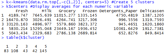
Now we can start interpreting the cluster results:
- Cluster 1 looks to be a heavy Grocery and above average Detergents_Paper but low Fresh foods.
- Cluster 3 is dominant in the Fresh category.
- Cluster 5 might be either the “junk drawer” catch-all cluster or it might represent the small customers.
A measurement that is more relative would be the withinss and betweenss.
- k$withinss would tell you the sum of the square of the distance from each data point to the cluster center. Lower is better. Seeing a high withinss would indicate either outliers are in your data or you need to create more clusters.
- k$betweenss tells you the sum of the squared distance between cluster centers. Ideally you want cluster centers far apart from each other.
It’s important to try other values for K. You can then compare withinss and betweenss. This will help you select the best K. For example, with this data set, what if you ran K from 2 through 20 and plotted the total within sum of squares? You should find an “elbow” point. Wherever the graph bends and stops making gains in withinss you call that your K.
rng<-2:20 #K from 2 to 20
tries <-100 #Run the K Means algorithm 100 times
avg.totw.ss <-integer(length(rng)) #Set up an empty vector to hold all of points
for(v in rng){ # For each value of the range variable
 v.totw.ss <-integer(tries) #Set up an empty vector to hold the 100 tries
 for(i in 1:tries){
 k.temp <-kmeans(data.rm.top,centers=v) #Run kmeans
 v.totw.ss[i] <-k.temp$tot.withinss#Store the total withinss
 }
 avg.totw.ss[v-1] <-mean(v.totw.ss) #Average the 100 total withinss
}
plot(rng,avg.totw.ss,type="b", main="Total Within SS by Various K",
 ylab="Average Total Within Sum of Squares",
 xlab="Value of K")
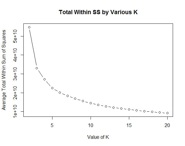
This plot doesn’t show a very strong elbow. Somewhere around K = 5 we start losing dramatic gains. So I’m satisfied with 5 clusters.
You now have all of the bare bones for using kmeans clustering in R.
Here’s the full code for this tutorial.
data <-read.csv("Wholesale customers data.csv",header=T)
summary(data)
top.n.custs <- function (data,cols,n=5) { #Requires some data frame and the top N to remove
idx.to.remove <-integer(0) #Initialize a vector to hold customers being removed
for (c in cols){ # For every column in the data we passed to this function
col.order <-order(data[,c],decreasing=T) #Sort column "c" in descending order (bigger on top)
#Order returns the sorted index (e.g. row 15, 3, 7, 1, ...) rather than the actual values sorted.
idx <-head(col.order, n) #Take the first n of the sorted column C to
idx.to.remove <-union(idx.to.remove,idx) #Combine and de-duplicate the row ids that need to be removed
}
return(idx.to.remove) #Return the indexes of customers to be removed
}
top.custs <-top.n.custs(data,cols=3:8,n=5)
length(top.custs) #How Many Customers to be Removed?
data[top.custs,] #Examine the customers
data.rm.top <-data[-c(top.custs),] #Remove the Customers
set.seed(76964057) #Set the seed for reproducibility
k <-kmeans(data.rm.top[,-c(1,2)], centers=5) #Create 5 clusters, Remove columns 1 and 2
k$centers #Display cluster centers
table(k$cluster) #Give a count of data points in each cluster
rng<-2:20 #K from 2 to 20
tries<-100 #Run the K Means algorithm 100 times
avg.totw.ss<-integer(length(rng)) #Set up an empty vector to hold all of points
for(v in rng){ # For each value of the range variable
v.totw.ss<-integer(tries) #Set up an empty vector to hold the 100 tries
for(i in 1:tries){
k.temp<-kmeans(data.rm.top,centers=v) #Run kmeans
v.totw.ss[i]<-k.temp$tot.withinss#Store the total withinss
}
avg.totw.ss[v-1]<-mean(v.totw.ss) #Average the 100 total withinss
}
plot(rng,avg.totw.ss,type="b", main="Total Within SS by Various K",
ylab="Average Total Within Sum of Squares",
xlab="Value of K")