KNN calculates the distance between a test object and all training objects.  Using the K nearest neighbors, we can classify the test objects.  The simplest kNN implementation is in the {class} library and uses the knn function.

Tutorial Time: 10 minutes

Classifying Irises with kNN

One of the benefits of kNN is that you can handle any number of classes.  A classic data mining data set created by R.A. Fisher.  It has three types of irises (Virginica, Setosa, and Versicolor), evenly distributed (50 each).  We’ll use the knn function to try to classify a sample of flowers.

We’ll start by loading the class library and splitting the iris data set into a training and test set.

library(class) #Has the knn function
set.seed(4948493) #Set the seed for reproducibility
#Sample the Iris data set (70% train, 30% test)
ir_sample<-sample(1:nrow(iris),size=nrow(iris)*.7)
ir_train<-iris[ir_sample,] #Select the 70% of rows
ir_test<-iris[-ir_sample,] #Select the 30% of rows

With the data separated, we can start trying different levels of K.  We’ll set up a holding variable (iris_acc) to store the performance at each K.  Then we’ll loop from 1 through 50 (i.e. number of neighbors) and then plot to see which one performs best.

iris_acc<-numeric() #Holding variable

for(i in 1:50){
 #Apply knn with k = i
 predict<-knn(ir_train[,-5],ir_test[,-5],
 ir_train$Species,k=i)
 iris_acc<-c(iris_acc,
 mean(predict==ir_test$Species))
}
#Plot k= 1 through 50
plot(1-iris_acc,type="l",ylab="Error Rate",
 xlab="K",main="Error Rate for Iris With Varying K")

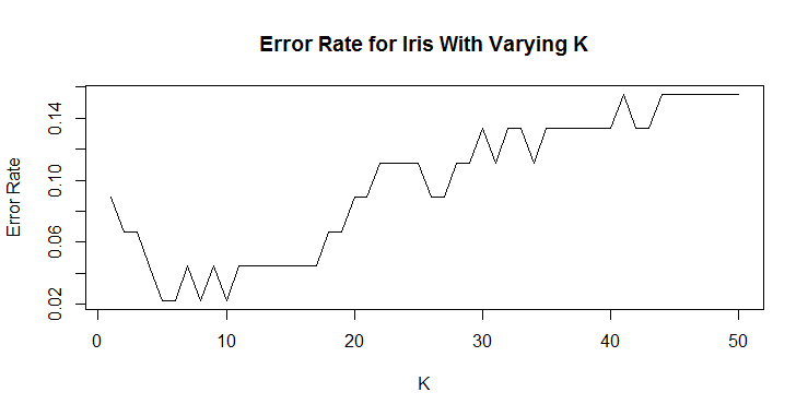
We can see that any number of neighbors beyond 10 appears to produce a less accurate classification.  We can (and should) run this many more times to make sure that our K is accurate.  We can run 100 samples of the iris data set and look at k = 1 through 20.  Much of the code for this section is very similar, just wrapped in a for loop.

trial_sum<-numeric(20)
trial_n<-numeric(20)
set.seed(6033850)
for(i in 1:100){
 ir_sample<-sample(1:nrow(iris),size=nrow(iris)*.7)
 ir_train<-iris[ir_sample,]
 ir_test<-iris[-ir_sample,]
 test_size<-nrow(ir_test)
 for(j in 1:20){
 predict<-knn(ir_train[,-5],ir_test[,-5],
 ir_train$Species,k=j)
 trial_sum[j]<-trial_sum[j]+sum(predict==ir_test$Species)
 trial_n[j]<-trial_n[j]+test_size
 }
}

plot(1-trial_sum / trial_n,type="l",ylab="Error Rate",
 xlab="K",main="Error Rate for Iris With Varying K (100 Samples)")

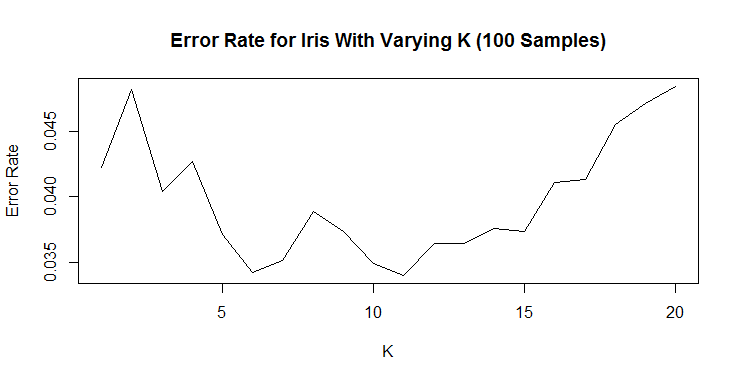
Now there is a clear pattern where less than 5 neighbors are too few and more than 11 neighbors quickly become too many.  For simplicity’s sake, I would choose 6 neighbors based on this chart.

Now, for any new iris we collect, we can quickly identify its species by taking the majority of its six closest neighbors.

Complete Code

#kNN Tutotrial on Iris Data Set####
library(class) #Has the knn function
set.seed(4948493) #Set the seed for reproducibility
#Sample the Iris data set (70% train, 30% test)
ir_sample<-sample(1:nrow(iris),size=nrow(iris)*.7)
ir_train<-iris[ir_sample,] #Select the 70% of rows
ir_test<-iris[-ir_sample,] #Select the 30% of rows

#First Attempt to Determine Right K####
iris_acc<-numeric() #Holding variable

for(i in 1:50){
 #Apply knn with k = i
 predict<-knn(ir_train[,-5],ir_test[,-5],
 ir_train$Species,k=i)
 iris_acc<-c(iris_acc,
 mean(predict==ir_test$Species))
}
#Plot k= 1 through 30
plot(1-iris_acc,type="l",ylab="Error Rate",
 xlab="K",main="Error Rate for Iris With Varying K")

#Try many Samples of Iris Data Set to Validate K####
trial_sum<-numeric(20)
trial_n<-numeric(20)
set.seed(6033850)
for(i in 1:100){
 ir_sample<-sample(1:nrow(iris),size=nrow(iris)*.7)
 ir_train<-iris[ir_sample,]
 ir_test<-iris[-ir_sample,]
 test_size<-nrow(ir_test)
 for(j in 1:20){
 predict<-knn(ir_train[,-5],ir_test[,-5],
 ir_train$Species,k=j)
 trial_sum[j]<-trial_sum[j]+sum(predict==ir_test$Species)
 trial_n[j]<-trial_n[j]+test_size
 }
}

plot(1-trial_sum / trial_n,type="l",ylab="Error Rate",
 xlab="K",main="Error Rate for Iris With Varying K (100 Samples)")