Summary: R linear regression uses the lm() function to create a regression model given some formula, in the form of Y~X+X2.  To look at the model, you use the summary() function.  To analyze the residuals, you pull out the $resid variable from your new model.  Residuals are the differences between the prediction and the actual results and you need to analyze these differences to find ways to improve your regression model.

To do linear (simple and multiple) regression in R you need the built-in lm function.

Here’s the data we will use, one year of marketing spend and company sales by month. Download: CSV

[table]Month,Spend,Sales
1,1000,9914
2,4000,40487
3,5000,54324
4,4500,50044
5,3000,34719
6,4000,42551
7,9000,94871
8,11000,118914
9,15000,158484
10,12000,131348
11,7000,78504
12,3000,36284[/table]

Assuming you’ve downloaded the CSV, we’ll read the data in to R and call it the dataset variable

#You may need to use the setwd(directory-name) command to
#change your working directory to wherever you saved the csv.
#Use getwd() to see what your current directory is.
dataset = read.csv("data-marketing-budget-12mo.csv", header=T,
colClasses = c("numeric", "numeric", "numeric"))

Simple (One Variable) and Multiple Linear Regression Using lm()

The predictor (or independent) variable for our linear regression will be Spend (notice the capitalized S) and the dependent variable (the one we’re trying to predict) will be Sales (again, capital S).

The lm function really just needs a formula (Y~X) and then a data source.  We’ll use Sales~Spend, data=dataset and we’ll call the resulting linear model “fit”.

simple.fit = lm(Sales~Spend, data=dataset)
summary(simple.fit)
multi.fit = lm(Sales~Spend+Month, data=dataset)
summary(multi.fit)

Notices on the multi.fit line the Spend variables is accompanied by the Month variable and a plus sign (+).  The plus sign includes the Month variable in the model as a predictor (independent) variable.

The summary function outputs the results of the linear regression model.

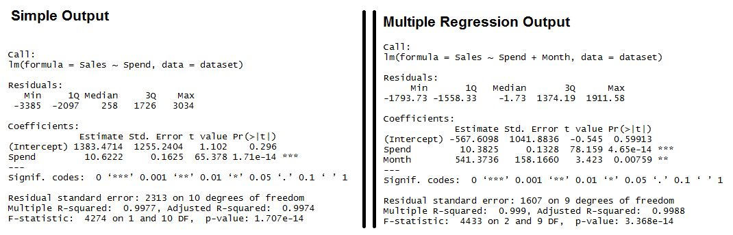
Output for R’s lm Function showing the formula used, the summary statistics for the residuals, the coefficients (or weights) of the predictor variable, and finally the performance measures including RMSE, R-squared, and the F-Statistic.

Both models have significant models (see the F-Statistic for Regression) and the Multiple R-squared and Adjusted R-squared are both exceptionally high (keep in mind, this is a simplified example).  We also see that all of the variables are significant (as indicated by the “**”)

Interpreting R’s Regression Output

• Residuals: The section summarizes the residuals, the error between the prediction of the model and the actual results.  Smaller residuals are better.
• Coefficients: For each variable and the intercept, a weight is produced and that weight has other attributes like the standard error, a t-test value and significance.
  • Estimate: This is the weight given to the variable.  In the simple regression case (one variable plus the intercept), for every one dollar increase in Spend, the model predicts an increase of $10.6222.
  • Std. Error: Tells you how precisely was the estimate measured.  It’s really only useful for calculating the t-value.
  • t-value and Pr(>[t]): The t-value is calculated by taking the coefficient divided by the Std. Error.  It is then used to test whether or not the coefficient is significantly different from zero.  If it isn’t significant, then the coefficient really isn’t adding anything to the model and could be dropped or investigated further.  Pr(>|t|) is the significance level.

• Performance Measures: Three sets of measurements are provided.
  • Residual Standard Error: This is the standard deviation of the residuals.  Smaller is better.
  • Multiple / Adjusted R-Square: For one variable, the distinction doesn’t really matter.  R-squared shows the amount of variance explained by the model.  Adjusted R-Square takes into account the number of variables and is most useful for multiple-regression.
  • F-Statistic: The F-test checks if at least one variable’s weight is significantly different than zero.  This is a global test to help asses a model.  If the p-value is not significant (e.g. greater than 0.05) than your model is essentially not doing anything.

Need more concrete explanations?  I explain summary output on this page.

With the descriptions out of the way, let’s start interpreting.

Residuals: We can see that the multiple regression model has a smaller range for the residuals: -3385 to 3034 vs. -1793 to 1911.  Secondly the median of the multiple regression is much closer to 0 than the simple regression model.

• Coefficients:
  • (Intercept): The intercept is the left over when you average the independent and dependent variable.  In the simple regression we see that the intercept is much larger meaning there’s a fair amount left over.  Multiple regression shows a negative intercept but it’s closer to zero than the simple regression output.
  • Spend: Both simple and multiple regression shows that for every dollar you spend, you should expect to get around 10 dollars in sales.
  • Month: When we add in the Month variable it’s multiplying this variable times the numeric (ordinal) value of the month.  So for every month you are in the year, you add an additional 541 in sales.  So February adds in $1,082 while December adds $6,492 in Sales.

• Performance Measures:
  • Residual Standard Error: The simple regression model has a much higher standard error, meaning the residuals have a greater variance.  A 2,313 standard error is pretty high considering the average sales is $70,870.
  • Multiple / Adjusted R-Square: The R-squared is very high in both cases.  The Adjusted R-square takes in to account the number of variables and so it’s more useful for the multiple regression analysis.
  • F-Statistic: The F-test is statistically significant.  This means that both models have at least one variable that is significantly different than zero.

Analyzing Residuals

Anyone can fit a linear model in R.  The real test is analyzing the residuals (the error or the difference between actual and predicted results).

There are four things we’re looking for when analyzing residuals.

• The mean of the errors is zero (and the sum of the errors is zero)
• The distribution of the errors are normal.
• All of the errors are independent.
• Variance of errors is constant (Homoscedastic)

In R, you pull out the residuals by referencing the model and then the resid variable inside the model.  Using the simple linear regression model (simple.fit) we’ll plot a few graphs to help illustrate any problems with the model.

layout(matrix(c(1,1,2,3),2,2,byrow=T))
#Spend x Residuals Plot
plot(simple.fit$resid~dataset$Spend[order(dataset$Spend)],
 main="Spend x Residuals\nfor Simple Regression",
 xlab="Marketing Spend", ylab="Residuals")
abline(h=0,lty=2)
#Histogram of Residuals
hist(simple.fit$resid, main="Histogram of Residuals",
 ylab="Residuals")
#Q-Q Plot
qqnorm(simple.fit$resid)
qqline(simple.fit$resid)

 Residuals are normally distributed

The histogram and QQ-plot are the ways to visually evaluate if the residual fit a normal distribution.

• If the histogram looks like a bell-curve it might be normally distributed.
• If the QQ-plot has the vast majority of points on or very near the line, the residuals may be normally distributed.

The plots don’t seem to be very close to a normal distribution, but we can also use a statistical test.

The Jarque-Bera test (in the fBasics library, which checks if the skewness and kurtosis of your residuals are similar to that of a normal distribution.

• The Null hypothesis of the jarque-bera test is that skewness and kurtosis of your data are both equal to zero (same as the normal distribution).

library(fBasics)
jarqueberaTest(simple.fit$resid) #Test residuals for normality
#Null Hypothesis: Skewness and Kurtosis are equal to zero
#Residuals X-squared: 0.9575 p Value: 0.6195

With a p value of 0.6195, we fail to reject the null hypothesis that the skewness and kurtosis of residuals are statistically equal to zero.

Residuals are independent

The Durbin-Watson test is used in time-series analysis to test if there is a trend in the data based on previous instances – e.g. a seasonal trend or a trend every other data point.

Using the lmtest library, we can call the “dwtest” function on the model to check if the residuals are independent of one another.

• The Null hypothesis of the Durbin-Watson test is that the errors are serially UNcorrelated.

library(lmtest) #dwtest
dwtest(simple.fit) #Test for independence of residuals
#Null Hypothesis: Errors are serially UNcorrelated
#Results: DW = 1.1347, p-value = 0.03062

Based on the results, we can reject the null hypothesis that the errors are serially uncorrelated.  This means we have more work to do.

Let’s try going through these motions for the multiple regression model.

layout(matrix(c(1,2,3,4),2,2,byrow=T))
plot(multi.fit$fitted, rstudent(multi.fit),
 main="Multi Fit Studentized Residuals",
 xlab="Predictions",ylab="Studentized Resid",
 ylim=c(-2.5,2.5))
abline(h=0, lty=2)
plot(dataset$Month, multi.fit$resid,
 main="Residuals by Month",
 xlab="Month",ylab="Residuals")
abline(h=0,lty=2)
hist(multi.fit$resid,main="Histogram of Residuals")
qqnorm(multi.fit$resid)
qqline(multi.fit$resid)

Residuals are Normally Distributed

• Histogram of residuals does not look normally distributed.
• However, the QQ-Plot shows only a handful of points off of the normal line.
• We fail to reject the Jarque-Bera null hypothesis (p-value = 0.5059)

library(fBasics)
jarqueberaTest(multi.fit$resid) #Test residuals for normality
#Null Hypothesis: Skewness and Kurtosis are equal to zero
#Residuals X-squared: 1.3627 p Value: 0.5059

Residuals are independent

• We fail to reject the Durbin-Watson test’s null hypothesis (p-value 0.3133)

library(lmtest) #dwtest
dwtest(multi.fit) #Test for independence of residuals
#Null Hypothesis: Errors are serially UNcorrelated
#Results: DW = 2.1077, p-value = 0.3133

Residuals have constant variance

Constant variance can be checked by looking at the “Studentized” residuals – normalized based on the standard deviation.  “Studentizing” lets you compare residuals across models.

The Multi Fit Studentized Residuals plot shows that there aren’t any obvious outliers.  If a point is well beyond the other points in the plot, then you might want to investigate.  Based on the plot above, I think we’re okay to assume the constant variance assumption.  More data would definitely help fill in some of the gaps.

Recap / Highlights

• Regression is a powerful tool for predicting numerical values.
• R’s lm function creates a regression model.
• Use the summary function to review the weights and performance measures.
• The residuals can be examined by pulling on the $resid variable from your model.
• You need to check your residuals against these four assumptions.
  • The mean of the errors is zero (and the sum of the errors is zero).
  • The distribution of the errors are normal.
  • All of the errors are independent.
  • Variance of errors is constant (Homoscedastic)

Here’s the full code below

dataset = read.csv("data-marketing-budget-12mo.csv", header=T,
colClasses = c("numeric", "numeric", "numeric"))
head(dataset,5)
#/////Simple Regression/////
simple.fit = lm(Sales~Spend,data=dataset)
summary(simple.fit)

#Loading the necessary libraries
library(lmtest) #dwtest
library(fBasics) #JarqueBeraTest

#Testing normal distribution and independence assumptions
jarqueberaTest(simple.fit$resid) #Test residuals for normality
#Null Hypothesis: Skewness and Kurtosis are equal to zero
dwtest(simple.fit) #Test for independence of residuals
#Null Hypothesis: Errors are serially UNcorrelated

#Simple Regression Residual Plots
layout(matrix(c(1,1,2,3),2,2,byrow=T))
#Spend x Residuals Plot
plot(simple.fit$resid~dataset$Spend[order(dataset$Spend)],
     main="Spend x Residuals\nfor Simple Regression",
     xlab="Marketing Spend", ylab="Residuals")
abline(h=0,lty=2)
#Histogram of Residuals
hist(simple.fit$resid, main="Histogram of Residuals",
     ylab="Residuals")
#Q-Q Plot
qqnorm(simple.fit$resid)
qqline(simple.fit$resid)

#///////////Multiple Regression Example///////////

multi.fit = lm(Sales~Spend+Month, data=dataset)
summary(multi.fit)

#Residual Analysis for Multiple Regression
dwtest(multi.fit) #Test for independence of residuals
#Null Hypothesis: Errors are serially UNcorrelated
jarqueberaTest(multi.fit$resid) #Test residuals for normality
#Null Hypothesis: Skewness and Kurtosis are equal to zero

#Multiple Regression Residual Plots
layout(matrix(c(1,2,3,4),2,2,byrow=T))
plot(multi.fit$fitted, rstudent(multi.fit),
     main="Multi Fit Studentized Residuals",
     xlab="Predictions",ylab="Studentized Resid",
     ylim=c(-2.5,2.5))
abline(h=0, lty=2)
plot(dataset$Month, multi.fit$resid,
     main="Residuals by Month",
     xlab="Month",ylab="Residuals")
abline(h=0,lty=2)
hist(multi.fit$resid,main="Histogram of Residuals")
qqnorm(multi.fit$resid)
qqline(multi.fit$resid)

Corrections:

• Thanks to Thiam Huat for the correction on coefficient interpretation.