Summary: The neuralnet package requires an all numeric input data.frame / matrix. You control the hidden layers with hidden= and it can be a vector for multiple hidden layers. To predict with your neural network use the compute function since there is not predict function.
Tutorial Time: 40 minutes
Libraries Needed: neuralnet
This tutorial does not spend much time explaining the concepts behind neural networks. See the method page on the basics of neural networks for more information before getting into this tutorial.
Data Needed: http://archive.ics.uci.edu/ml/datasets/Bank+Marketing (bank.Zip)
neuralnet(formula, data, hidden = 1,
 threshold = 0.01, stepmax = 1e+05,
 rep = 1, startweights = NULL,
 learningrate.limit = NULL,
 learningrate.factor =
     list(minus = 0.5, plus = 1.2),
 learningrate=NULL, lifesign = "none",
 lifesign.step = 1000, algorithm = "rprop+",
 err.fct = "sse", act.fct = "logistic",
 linear.output = TRUE, exclude = NULL,
 constant.weights = NULL, likelihood = FALSE)
Data Understanding
It’s important to note that the neuralnet package requires numeric inputs and does not play nicely with factor variables. As a result, we need to investigate which variables need to be transformed.
We can get an overall structure of our data by using str()
str(bnk)
'data.frame':	4521 obs. of  17 variables:
 $ age      : int  30 33 35 30 59 35 36 39 41 43 ...
 $ job      : Factor w/ 12 levels "admin.","blue-collar",..: 11 8 5 5 2 5 7 10 3 8 ...
 $ marital  : Factor w/ 3 levels "divorced","married",..: 2 2 3 2 2 3 2 2 2 2 ...
 $ education: Factor w/ 4 levels "secondary","primary",..: 2 1 3 3 1 3 3 1 3 2 ...
 $ default  : Factor w/ 2 levels "no","yes": 1 1 1 1 1 1 1 1 1 1 ...
 $ balance  : int  1787 4789 1350 1476 0 747 307 147 221 -88 ...
 $ housing  : Factor w/ 2 levels "no","yes": 1 2 2 2 2 1 2 2 2 2 ...
 $ loan     : Factor w/ 2 levels "no","yes": 1 2 1 2 1 1 1 1 1 2 ...
 $ month    : Factor w/ 12 levels "apr","aug","dec",..: 11 9 1 7 9 4 9 9 9 1 ...
 $ campaign : int  1 1 1 4 1 2 1 2 2 1 ...
 $ poutcome : Factor w/ 4 levels "failure","other",..: 4 1 1 4 4 1 2 4 4 1 ...
 $ y        : Factor w/ 2 levels "no","yes": 1 1 1 1 1 1 1 1 1 1 ...
As neural networks use activation functions between -1 and +1, it’s important to scale your variables down. Otherwise, the neural network will have to spend training iterations doing that scaling for you.
#Min Max Normalization
bnk$balance <-(bnk$balance-min(bnk$balance)) /
                  (max(bnk$balance)-min(bnk$balance))
bnk$age <- (bnk$age-min(bnk$age)) / (max(bnk$age)-min(bnk$age))
bnk$previous <- (bnk$previous-min(bnk$previous)) /
                  (max(bnk$previous)-min(bnk$previous))
bnk$campaign <- (bnk$campaign-min(bnk$campaign)) /
                  (max(bnk$campaign)-min(bnk$campaign))
neuralnet and the model.matrix function
In order to represent factor variables, we need to convert them into dummy variables. A dummy variable takes the N distinct values and converts it into N-1 variables. We use N-1 because the final value is represented by all dummy values set to zero.
For any given row either one or none of the dummy variables will be active with a one (1) or inactive with zero (0).
In our bank data set, the variable education has four distinct values with “primary” being the base case (i.e. the first level)
table(bnk$education)
#  primary secondary  tertiary   unknown
#      678      2306      1350       187
levels(bnk$education)
#[1] "primary"   "secondary" "tertiary"  "unknown"
In order to make this factor variable useful for the neuralnet package, we need to use the model.matrix() function.
head(model.matrix(~education, data=bnk))
#  (Intercept) educationsecondary educationtertiary educationunknown
#1      1      0      0      0
#2      1      1      0      0
#3      1      0      1      0
The model.matrix function split the education variable into all possible values except the base case. It adds an intercept variable which we will eventually drop. If you wanted to include that particular value, you need to relevel() your data.
bnk$education <- relevel(bnk$education, ref = "secondary")
head(model.matrix(~education, data=bnk))
#  (Intercept) educationprimary educationtertiary educationunknown
#1   1      1      0      0
#2   1      0      0      0
#3   1      0      1      0
Once we have decided on all of our numeric and factor variables, we can call the function one last time.
bnk_matrix <- model.matrix(~age+job+marital+education
                           +default+balance+housing
                           +loan+poutcome+campaign
                           +previous+y, data=bnk)
We now have a matrix with 28 columns (27 excluding the intercept). Using this new variable, we can start building our neural networks.
Before we get to model building, we need to make sure all of the column names are acceptable model inputs. It looks like two columns have special characters and we need to fix that before entering it into a model.
colnames(bnk_matrix)
# [1] "(Intercept)"        "age"                "jobblue-collar"
# [4] "jobentrepreneur"    "jobhousemaid"       "jobmanagement"
# [7] "jobretired"         "jobself-employed"   "jobservices"
colnames(bnk_matrix)[3] <- "jobbluecollar"
colnames(bnk_matrix)[8] <- "jobselfemployed"
Now that we have all of the column names cleaned up, we need to get it into a formula. We have to combine the column names (separated by a plus symbol) and then tack on the response variable.
col_list <- paste(c(colnames(bnk_matrix[,-c(1,28)])),collapse="+")
col_list <- paste(c("yyes~",col_list),collapse="")
f <- formula(col_list)
Finally, we’re ready to use this formula in our models.
Modeling
With the complexity of neural networks, there are lots of options to explore in the neuralnet package. We’ll start with the default parameters and then explore a few different options.
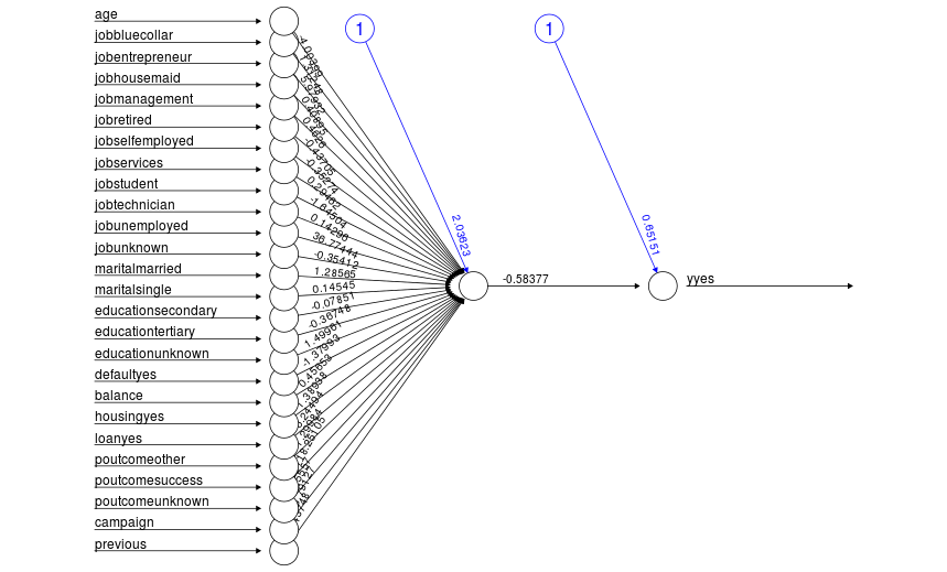
Default Neural Network With One Hidden Node (RPROP+)
library(neuralnet)
set.seed(7896129)

nmodel <- neuralnet(f,data=bnk_matrix,hidden=1,
                    threshold = 0.01,
                    learningrate.limit = NULL,
                    learningrate.factor =
                         list(minus = 0.5, plus = 1.2),
                    algorithm = "rprop+")
- By default, you’re using the Resilient Backpropogation algorithm (RPROP+).
- This requires a
learningrate.limitandlearningrate.factor. - The LIMIT sets the upperbound that the learning rate could reach.
- The rate factor is the multiplier that the rate will change if…
minus: the model has jumped over the local minima.plus: the model is going in the right direction.
RPROP is a fast algorithm and doesn’t require as much tuning as classic backpropogation since you’re not setting a static learning rate. Instead, the learningrate.factor.
But as usual, you can accept the default parameters and your cod will work!
Changing Hidden Nodes and Backprop
A neural network with a single hidden node isn’t anything better than a linear combination really. In order to change the number of hidden nodes, we simply use the hidden parameter.
##### Varying RPROP Hidden Nodes and Repetitions
set.seed(7896129)
nn5 <- neuralnet(f,data=bnk_matrix,hidden=5)
Easy.
Now what if we wanted to change the algorithm? That requires adjusting some of the parameters.
#This results in an error!!
nn_backprop <- neuralnet(f, data=bnk_matrix,
                          algorithm = "backprop")
#Error: 'learningrate' must be a numeric value, if the #backpropagation algorithm is used

#This works (but likely won't converge)!
nn_backprop <- neuralnet(f, data=bnk_matrix,
                         algorithm = "backprop",
                         learningrate = 0.0001)
The important parameter for backprop is the learningrate which is called “alpha” in the classic description of backprop.
An important note is that you need to set the learningrate small enough or you will run into this error
Error in if (reached.threshold < min.reached.threshold) { :
  missing value where TRUE/FALSE needed
The best solution I have found is to just keep the learningrate very small.
Multiple Hidden Layers

Deep Learning is partially about having multiple hidden layers in a neural network. The neuralnet package allows you to change the hidden parameter to a vector.
#RPROP Multiple layers
set.seed(1973549813)

nn_rprop_multi <- neuralnet(f, data=bnk_matrix,
                         algorithm = "rprop+",
                         hidden=c(10,3),
                         threshold=0.1,
                         stepmax = 1e+06)
If your model converges or you have some parallel processing abilities, it's worth experimenting with multi-level neural networks.
Some Advanced Features
There are a handful of other parameters that are worth looking at.
thresholdBy default, neuralnet requires the model partial derivative error to change at least 0.01 otherwise it will stop changing.stepmaxwill control how long your neural network trains. By default, it uses 100,000 iterations.startweightsis a vector of weights you want to start from. You could use this as a way of using an existing neural network and updating the weights.lifesignandlifesign.stepprovide an update for you as sit and wait for your model to finish. The "full" lifesign looks like this...
hidden: 10    thresh: 0.1    rep: 1/1
steps:    1000	min thresh: 0.5792730128
2000	min thresh: 0.4859884745
3000	min thresh: 0.4276816262
4000	min thresh: 0.4276816262
5000	min thresh: 0.4267513944
...
Another parameter that I wanted to explain in a little more detail is the rep parameter. The rep allows you to repeat your training with different starting weights (assuming you haven't defined them already).
By defining rep=5, you will get the results from 5 different neural networks.
#Creating a neural network stopped at threshold = 0.5
nn_rprop_rep5 <- neuralnet(f, data=bnk_matrix,
                           algorithm = "rprop+",
                           hidden=c(15),
                           threshold=0.5,
                           rep=5,
                           stepmax = 1e+06)
nn_rprop_rep5
5 repetitions were calculated.

        Error Reached Threshold Steps
4 166.1777017      0.4936484239  5613
2 166.5174888      0.4444659596  6887
5 169.9497032      0.4721955880  4167
3 173.3583823      0.4495817644  3043
1 175.6160528      0.4841837841  3205
If you go to visualize your neural network that used repetitions, be warned that, by default, it will print every repetition that converged. You can control the plotting by using the rep parameter. plot(nn_rprop_rep5, rep = 4)
How to Predict With neuralnet (use compute)
For some reason, the authors of this package decided to ignore the standard predict function and instead use compute instead.
output <- compute(nmodel, bnk_matrix[,-c(1,28)],rep=1)
summary(output)
#           Length Class  Mode
#neurons       2   -none- list
#net.result 4521   -none- numeric
Important notes on the compute function.
- Do not pass any extra data when predicting. Otherwise you'll receive the error
Error in neurons[[i]] %*% weights[[i]] : non-conformable arguments. - Make sure you set up your train and test data in a similar way.
- In this example, I had to remove the first and 28th column to make it match the training data
- If you used multiple repetitions (
rep=) when training, you can specify which result to use. Otherwise it defaults to the first - The output of compute produces...
neurons: A list containing the weights between each node for each layer.net.result: The predictions for each test input. This is what you really want.- If your neural network has multiple outputs, you'll receive a matrix with a column for each output node.
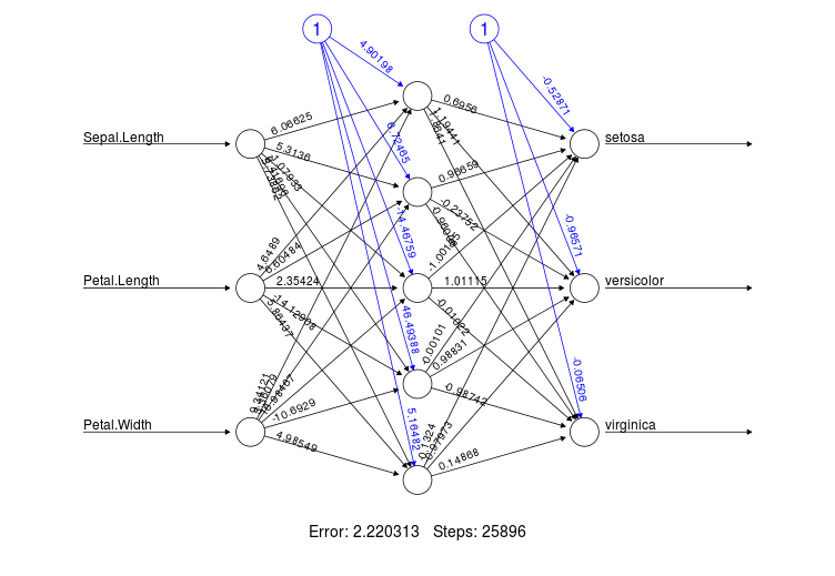
Training a Multi-Class Neural Network
In all honesty, I had to google this and I saw this StackOverflow post and I wanted to expand on it slightly.
If you want to predict multiple classes with one neural network, you simply have to define your formula and create dummy variables for each class. Here is my quick and dirty solution.
data(iris)
#Add a "fake" class to allow for all factors
levels(iris$Species) <- c(levels(iris$Species),"fake")
#Relevel to make the fake class the factor
iris$Species <- relevel(iris$Species,ref = "fake")
#Create dummy variables and remove the intercept
iris_multinom <- model.matrix(~Species+Sepal.Length+
                                Petal.Length+Petal.Width,
                              data=iris)[,-1]

colnames(iris_multinom)[1:3] <- c("setosa","versicolor","virginica")


nn_multi <- neuralnet(setosa+versicolor+virginica~
                 Sepal.Length+Petal.Length+Petal.Width,
               data=iris_multinom,hidden=5,lifesign = "minimum",
               stepmax = 1e+05,rep=10)
res <- compute(nn_multi, iris_multinom[,-c(1:3)])
Interpreting neuralnet Output
Lastly, there are some attributes you might want to keep around after you have built a neural network model.
model$weightsis a list that contains a nested list of matrices where each level is one layer. The list contains a nested list for every repetition.model$result.matrixis a collapsed version of the weight results with names like "variablex.to.1layhid1". There is a column for every repetition
That's It!
You now know just about everything on using the neuralnet package in R. There are lots of different parameters to mess around with and you can generate quite a few complicated neural network layouts with a few simple commands.