Autocorrelation is a way of identifying if a time series data set is correlated with a version of itself set off by a certain number of unit.
The equation of the sample autocorrelation function is:
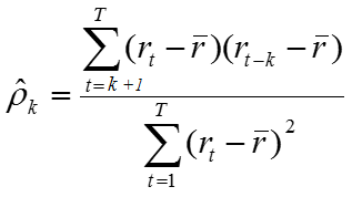
The top portion is essentially the covariance between the original data and the k-unit lagged data. The bottom is sum of the squared deviations of the original data set.
Variables Explained:
- r(t) = Your data set sorted by ascending date.
- r(t-k) = Same data set as above, but just shifted by k units.
- r_bar = The average of the original data set.
Examples by Hand: Let’s try calculating the Lag 3 Autocorrelation for the sample dataset below. This data has 24 observations (two years of monthly sales data).
| Original Data | 1-Unit Lag | 2-Unit Lag | 3-Unit Lag |
| 9.08 | |||
| 12.63 | 9.08 | ||
| 15.00 | 12.63 | 9.08 | |
| 20.73 | 15 | 12.63 | 9.08 |
| 2.20 | 20.73 | 15 | 12.63 |
| 18.00 | 2.2 | 20.73 | 15 |
| 7.16 | 18 | 2.2 | 20.73 |
| 18.28 | 7.16 | 18 | 2.2 |
| 21.00 | 18.28 | 7.16 | 18 |
| 19.68 | 21 | 18.28 | 7.16 |
| 15.54 | 19.68 | 21 | 18.28 |
| 24.00 | 15.54 | 19.68 | 21 |
| 16.10 | 24 | 15.54 | 19.68 |
| 11.93 | 16.1 | 24 | 15.54 |
| 27.00 | 11.93 | 16.1 | 24 |
| 12.51 | 27 | 11.93 | 16.1 |
| 20.04 | 12.51 | 27 | 11.93 |
| 30.00 | 20.04 | 12.51 | 27 |
| 12.41 | 30 | 20.04 | 12.51 |
| 14.33 | 12.41 | 30 | 20.04 |
| 33.00 | 14.33 | 12.41 | 30 |
| 22.11 | 33 | 14.33 | 12.41 |
| 17.91 | 22.11 | 33 | 14.33 |
| 36.00 | 17.91 | 22.11 | 33 |
- Original data’s Average = 18.1933
- Original data Sum of Squared Deviation = 1,455.431
Next, take the first column (original data) and subtract the original data’s average from each row, starting with the fourth row of data. Store that in its own column.
Then, take the fourth column (3-Unit Lag) and subtract the original data’s average from each row, starting with the fourth row of data. Store that in its own column as well.
For each row (21 in total) of the new columns, multiply the two values together. Add all 21 multiplications together. Finally, divide by the original data’s sum of squared deviations.
You’ll end up with: 647.8286 / 1455.431 = 0.4451112
This shows that there is 0.45 correlation with every three time units (months in this case). This could be a sign of seasonality in buyer behavior or some business event happening regularly every three months that influence sales.. For example, every three months (March, June, September and December) your company releases a new product which all your customers want to buy right away.
ACF in R:
All of that manual calculation can be done very easily in R with the acf function.
acf(original_data, lag=3, plot=F)
Autocorrelations of series ‘original_data’, by lag
| 0 | 1 | 2 | 3 |
| 1.000 | -0.093 | 0.039 | 0.445 |
- R calculates the acf for every integer between 0 and your designated lag.
- A lag of zero is perfectly correlated since it’s putting the exact same data against itself.
- If you set plot = T you’ll receive a correlogram for each lag with correlation on the y axis and number of units lagged on the y axis.
Hat Tip:
- DePaul University’s CSC 425 Time Series Analysis
- An Introduction to Analysis of Financial Data with R by Ruey S. Tsay