K-Means Clustering – What it is and How it Works

K-means clustering uses “centroids”, K different randomly-initiated points in the data, and assigns every data point to the nearest centroid. After every point has been assigned, the centroid is moved to the average of all of the points assigned to it. Then the process repeats: every point is assigned to its nearest centroid, centroids are moved to the average of points assigned to it. The algorithm is done when no point changes assigned centroid.

What is K-means Clustering

Clustering, in general, is an “unsupervised learning” method. That means we don’t have a target variable. We’re just letting the patterns in the data become more apparent.

K-means clustering distinguishes itself from Hierarchical since it creates K random centroids scattered throughout the data. The algorithm looks a little bit like…

Initialize K random centroids.
- You could pick K random data points and make those your starting points.
- Otherwise, you pick K random values for each variable.
For every data point, look at which centroid is nearest to it.
- Using some sort of measurement like Euclidean or Cosine distance.
Assign the data point to the nearest centroid.
For every centroid, move the centroid to the average of the points assigned to that centroid.
Repeat the last three steps until the centroid assignment no longer changes.
- The algorithm is said to have “converged” once there are no more changes.

These centroids act as the average representation of the points that are assigned to it. This gives you a story almost right away. You can compare the centroid values and tell if one cluster favors a group of variables or if the clusters have logical groupings of key variables.

Visualizing K-means Clustering

K-means clustering produces a very nice visual so here is a quick example of how each step might look.

method-k-means-steps-initial

Here’s 50 data points with three randomly initiated centroids.

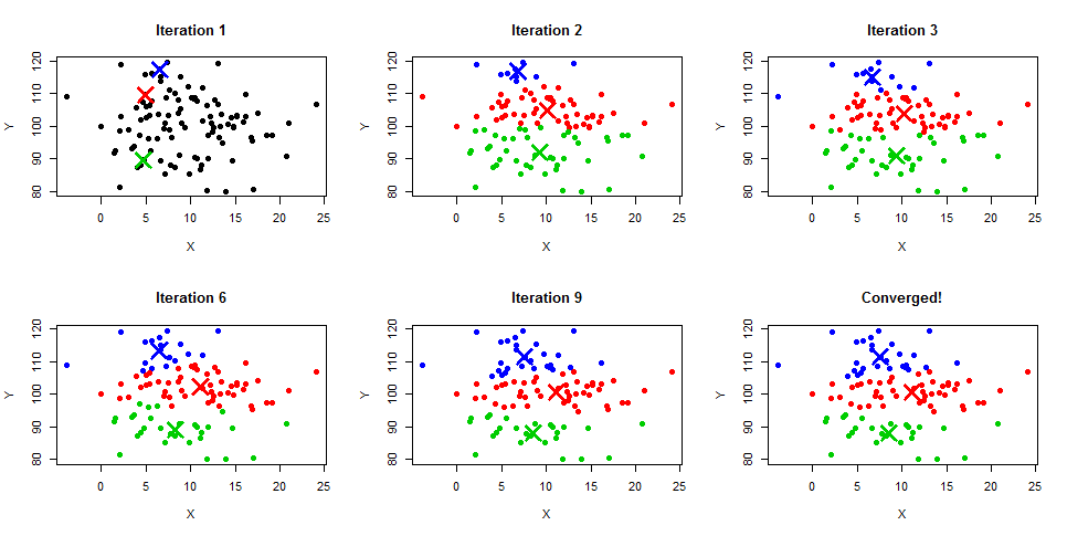
Iteration 2 shows the new location of the centroid centers.
Iteration 3 has a handful more blue points as the centroids move.
Jumping to iteration 6, we see the red centroid has moved further to the right.
Iteration 9 shows the green section is much smaller than in iteration 2, blue has taken over the top, and the red centroid is thinner than in iteration 6.
The 9th iteration’s results were the same as the 8th iteration’s, so it has “converged”.

Pre-processing and Things to Consider for K-means Clustering

There are a handful of pitfalls of k-means clustering that you should address.

Bigger values carry more weight.

This is a problem since not all of your data will be on the same scale. If you’re looking at a data set of real estate listings, the last purchase price and the number of bathrooms will be dramatically different. The distance between purchase prices will carry more weight.

The solution is to do some sort of normalization – minmax-normalization or z-score normalization are some fairly common options.

More variables pull data points further apart.

Imagine you’re in Seattle and you want to go to Mount Rainier. If you could go in a straight line, as the crow files, it’s around 50+ miles. Not too bad in two dimension (X and Y, two variables). But what if you’d like to get to the top of Mount Rainier. Well that’s another dimension (X, Y, and now Z).

If you wanted to get to the top of Mt. Rainier (elevation of 14,409 ft. above sea level) from Seattle (177 ft. above sea level), you’d travel around 14,200 feet (the diagonal line). If all three of these variables are in the k-means algorithm, it will seem twice as far apart than using only the two variables.

This happens all the time with real data. Throwing every variable in (even after normalizing) can create wide distance between otherwise close data points.

The solution is to do data reduction (such as principal components analysis) to create new variables that are more compact with data or do some variable selection (such as decision trees or forward-selection) to just drop variables that aren’t very important / predictive if you have a response variable.

For more on extra-dimensional space…

Carl Sagan’s experiences in flatland (YouTube).
How to Walk Through Walls in the 4th Dimension (YouTube)

Works Best on Numeric Data

Since the k-means algorithm computes the distance between two points, you can’t really do that with categorical (low, medium, high) variables.

A simple workaround for multiple categorical variables is to calculate the percent of times each variable matches in comparison to the cluster centroid.

Measuring Performance of K-means

Homogeneity and Completeness – If you have pre-existing class labels that you’re trying to duplicate with k-means clustering, you can use two measures: homogeneity and completeness.

Homogeneity means all of the observations with the same class label are in the same cluster.
Completeness means all members of the same class are in the same cluster.
Scikit-Learn (Python) has an excellent write-up on these two measures.

WithinSS – The Within sum of squares measures the sum of the squared difference from the cluster center. A smaller WithinSS (or SSW) means there is less variance in that cluster’s data. Here’s an example set of clusters and their data.

[table]Cluster,X,Y,Cluster VAR X,Cluster VAR Y,Var SUM
A,5,10,0.063,0.063,0.125
A,7,12,3.063,5.063,8.125
A,4,8,1.563,3.063,4.625
A,5,9,0.063,0.563,0.625
B,2,6,0.000,0.063,0.063
B,1,4,1.000,3.063,4.063
B,2,7,0.000,1.563,1.563
B,3,6,1.000,0.063,1.063
C,9,19,0.111,4.000,4.111
C,9,21,0.111,0.000,0.111
C,10,23,0.444,4.000,4.444
Avg A,5.25,9.75,,SSW A,13.500
Avg B,2,5.75,,SSW B,6.750
Avg C,9.33,21,,SSW C,8.667[/table]

The Cluster VAR X takes each row and subtracts it from its respective cluster’s average for X.
The same goes for Cluster VAR Y.
The Var SUM adds up the two Cluster VAR columns.
At the bottom, SSW (A, B, C) adds up the rows for its respective cluster.
We see that the WithinSS for cluster…
- A = 13.5
- B = 6.75
- C = 8.667
The TOTAL WithinSS is the sum of those three values. 13.5+6.47+8.667 = 28.637
The TotalSS (Total Sum of Squares) is same process ignoring the cluster groupings.
- For the table above, the Total sum of squares would be 536.182

How to Choose K (# of Clusters)

You can use the Total Within SS to compare different K’s. Trying several different K’s (2 clusters, 3 clusters, 4 clusters… N clusters), you plot their total within sum of squares and then look for an elbow in the graph.

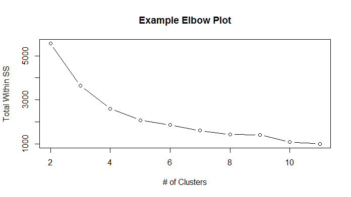
Plot showing change in Total Within Sum of Squares for K from 2 to 11

While not perfect, you can definitely see a flattening out around 7 or 8 clusters.
You may want to run this plot several times due to the random initialization of starting centroids.

Choosing SQRT(N / 2) clusters is a quick rule of thumb. If you have 100 data points, you could start off with SQRT(100/2) = SQRT(50) = 7 clusters.

The expectation is that each cluster will have SQRT(2*N) points.
In our example, we expect each cluster to have around SQRT(2*100) = SQRT(200) = 14 data points.
More information can be found in Data Mining Concepts and Techniques (3e.) Chapter 10

Learn by Marketing

Data Mining + Marketing in Plain English