There are two parts to this tutorial – part 1 will be manually calculating the simple linear regression coefficients “by hand” with Excel doing some of the math and part 2 will be actually using Excel’s built-in linear regression tool for simple and multiple regression.

Get the data – 12 Month Marketing Budget and Sales: CSV | XSLX

Jump to Using Excel’s Regression Tool

Simple Linear Regression Math by Hand

There are just a handful of steps in linear regression.

1. Calculate average of your X variable.
2. Calculate the difference between each X and the average X.
3. Square the differences and add it all up.  This is SSxx.
4. Calculate average of your Y variable.
5. Multiply the differences (of X and Y from their respective averages) and add them all together.  This is SSxy.
6. Using SSxx and SSxy, you calculate the intercept by subtracting SSxx / SSxy * AVG(X) from AVG(Y).

Using the example dataset, here are the calculations.

[table]Month,Spend,Avg(X) – X,(Avg(X)-X)^2,Sales,Avg(Y)-Y,(Avg(X)-X) * (Avg(Y)-Y)
1,1000,5541.67,”30,710,069.44″,9914,60956.33,”337,799,680.56″
2,4000,2541.67,”6,460,069.44″,40487,30383.33,”77,224,305.56″
3,5000,1541.67,”2,376,736.11″,54324,16546.33,”25,508,930.56″
4,4500,2041.67,”4,168,402.78″,50044,20826.33,”42,520,430.56″
5,3000,3541.67,”12,543,402.78″,34719,36151.33,”128,035,972.22″
6,4000,2541.67,”6,460,069.44″,42551,28319.33,”71,978,305.56″
7,9000,-2458.33,”6,043,402.78″,94871,-24000.67,”59,001,638.89″
8,11000,-4458.33,”19,876,736.11″,118914,-48043.67,”214,194,680.56″
9,15000,-8458.33,”71,543,402.78″,158484,-87613.67,”741,065,597.22″
10,12000,-5458.33,”29,793,402.78″,131348,-60477.67,”330,107,263.89″
11,7000,-458.33,”210,069.44″,78504,-7633.67,”3,498,763.89″
12,3000,3541.67,”12,543,402.78″,36284,34586.33,”122,493,263.89″
AVG,6541.67,,,70870.33,,
SUM,,,202729166.67,,,2153428833.33[/table]

The sum fields are our SSxx and SSxy (respectively).  To calculate our regression coefficient we divide the covariance of X and Y (SSxy) by the variance in X (SSxx)

Slope = SSxy / SSxx = 2153428833.33 / 202729166.67 = 10.62219546

The intercept is the “extra” that the model needs to make up for the average case.

Intercept = AVG(Y) – Slope * AVG(X)

Intercept = 70870.33 – 10.62219546 * 6541.67 = 1,383.471380

We now have our simple linear regression equation.

Y = 1,383.471380 + 10.62219546 * X

Doing Simple and Multiple Regression with Excel’s Data Analysis Tools

Excel makes it very easy to do linear regression using the Data Analytis Toolpak.

If you don’t have the Toolpak (seen in the Data tab under the Analysis section), you may need to add the tool.

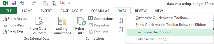
• Go to the Data tab, right-click and select Customize the Ribbon.

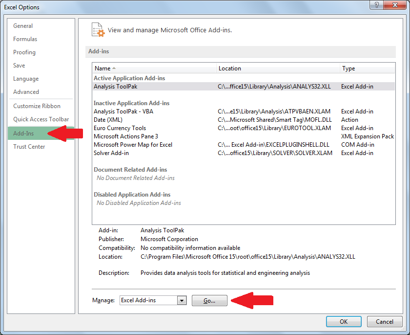
• Select the Add-ins section and go to Manage Excel Add-ins.
• You’ll then select the Analysis Toolpak and it should now be visible in the Data tab.

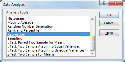
Now that we can select different built-in analyses, we’ll launch the regression tool.

If you’re using the CSV or XSLX file, you should mirror these options.

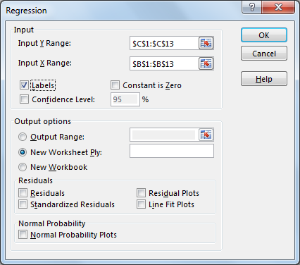
• Input Y Range is where the response variable (Sales in our case) is located.
• Input X Range is the range of predictor variables (Spend).
  • If there were additional X variables, they would all have to be next to each other.  No gaps between X variables allowed.
• Labels being checked means you have a header at the top of your X and Y range.

Additional options we haven’t checked are…

• Confidence Level – Adds another confidence interval at selected confidence level.
• Constant is Zero – Forces the X coefficient to capture more of the error.
  • Almost no reason to ever use this option unless your data has a theoretical reason to pass through the origin.
  • The regression equation is fundamentally changed as well (PDF Notes)
• Residuals – For every row, it provides the error / difference between predicted and actual values.
  • Standardized Residuals is normalized with mean zero and standard deviation of one.
  • Residual Plots charts the residuals by each variable.
  • Line Fit Plot charts the predicted results and the actual results by each variable
• Normal Probability Plots – Checks normality of your data.  Should see something close to a straight line.

Once you run the Excel Regression tool, we get…

• Regression Statistics – R-Squared stats and standard error
• ANOVA – Testing if the model is significant.
• Variable weights and statistics – Gives you the coefficient weights, p-value, and confidence bounds for the coefficients.

You now know how to do linear regression in Excel!  However, Excel is not the best tool to be using for data mining.  Try open source R and doing linear regression in R.