Summary: Logistic Regression is a tool for classifying and making predictions between zero and one. Coefficients are long odds. Odds are relative so when interpreting coefficients you need to set a baseline to compare in both numeric and categorical variables.
What is the probability that your customer will return next year? What has a greater impact on conversion rates: source of acquisition or time on site? These binary / probabilistic questions can be answered by logistic regression. Logistic regression…
- Is used in classification problems like retention, conversion, likelihood to purchase, etc.
- Can use continuous (numeric) or categorical (buckets / categories) as independent variables (inputs to the model).
- Has a binary (0 / 1) dependent variable (variable you’re trying to predict).
- Should not be trained on data with perfect separation (it breaks the mathematical underpinnings).
Logistic Regression Overview
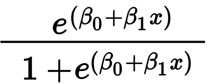
Logistic regression is similar to linear regression but it uses the traditional regression formula inside the logistic function of e^x / (1 + e^x). As a result, this logistic function creates a different way of interpreting coefficients.
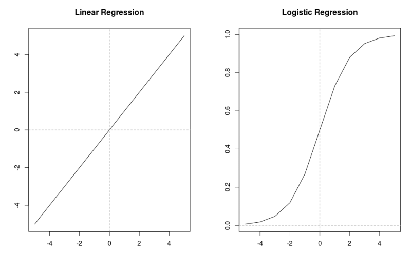
Visually, linear regression fits a straight line and logistic regression (probabilities) fits a curved line between zero and one. Notice in the image below how the inputs (x axis) are the same but the outputs (y axis) are dramatically different.
Logistic regression is a specific form of the “generalized linear models” that requires three parts.
- A dependent variable distribution (sometimes called a family).
- A mean function that is used to create the predictions.
- A link function that converts the mean function output back to the dependent variable’s distribution.
For logistic regression we work with…
- A binomial distribution (0 / 1).
- MeanFunc(x) = e^x / (1 + e^x)
- LinkFunc(u) = ln( u / (1 + u) )
The mean function is the logistic function and the link function is the logit equation. When working with tools like Python, R, and SAS, you need only to know that you’re doing a generalized linear model with a binomial distribution. The mean and link functions as described above are the defaults and the software knows this.
If you are given a logistic regression model and you want to generate values by hand, you’ll need to go through the steps below to get something easier to interpret.
Interpreting Logistic Regression Coefficients
For a deeper understanding of the relationship between log odds, odds, and probabilities, see this article on interpreting the log odds.
Since we are using logistic regression and not linear regression, the coefficients are the log odds. Plugging your values into the logistic regression equation won’t give you probabilities, instead it will give you the (natural) log odds value for your given data. Do not try to interpret the log odds. Instead, interpret the odds by taking e (euler’s number) raised to the log odds. That returns just the odds.
So what are odds?
The Odds from logistic regression is the exponential increase for any one unit. Let’s look at this with an example:
Let’s say we had a data set and logistic regression coefficients that looked like this:
acqSource = Google, Bing, Bing, Google, Google, Bing, Bing, Bing, Bing, Google
Convert = 0, 1, 0, 1, 1, 0, 0, 1, 1, 1

Intercept      acqSourceGoogle
7.401485e-17     1.098612

Odds of acqSourceGoogle = e^1.098612 = 3
Remember, the coefficients are the log odds. To really interpret them, we need to take e raised to the acqSourceGoogle coefficient. e^acqSourceGoogle is equal to 3. So we can say the odds of having a positive result given Google is 3:1 (read as 3 to 1). But 3:1 versus what? Versus Bing. We can say that being acquired by Google makes you three times more likely to convert than coming from Bing.
If we had three categories, each category would compare itself against the ‘base case’. Imagine we collected more data and had three categories of acquisition: Bing, Google, and Amazon. Further imagine that Bing is still our base case. The logistic regression output might look like this:
Intercept      acqSourceGoogle acqSourceAmazon
 2.543e-16     1.098612        1.386294

Odds of acqSourceGoogle = e^1.098612 = 3
Odds of acqSourceAmazon = e^1.386294 = 4
In comparison to the base case of Bing, customers acquired via Google are three times more likely than Bing to convert, customers acquired via Amazon are four times more likely than Bing to convert. This regression says nothing about the relationship between Google and Amazon though. To understand that, we would need to re-run the regression with the base case as Google.
What about numeric values? It’s a slightly different story.
As explained in my post on interpreting the log odds, the classic phrase “a one unit increase in X results in a Y increase in the dependent variable” doesn’t work the same way in logistic regression.
- The phrase is still true if you’re looking at log odds.
- If you are looking at the odds (e^log odds) it’s an exponential and relative effect.
- A one unit increase is different based on the value you’re increasing from!
- This means the increase depends on where you started. The increase from 1 to 2 is different than 2 to 3.
Ultimately, it comes down to the fact that you cannot interpret the odds the same way you do in linear regression. I suggest providing example points that make sense. For example, you might say an increase from 2 to 3 has 10x increase in the odds while a 3 to 4 increase has a 2x increase in the odds.
A quick rule of thumb to help interpretation is that if the odds are greater than one (i.e. after raising e to the log odds), there’s a direct relationship between your independent and dependent variable. If the odds are less than one, there’s an inverse / negative relationship. If they are equal to one, there’s no relationship.
Making Predictions With Logistic Regression
As mentioned above, logistic regression has coefficients in the form of the log odds. Thus, when you plug a new data point into the model you will get… a log odds value!
So we need to transform these values into something useful: probabilities.
The steps are as follows:
- Enter new data into logistic regression equation. Get log odds.
- Use the link function by first raising e to the log odds value (e ^ log odds). Get odds.
- Finish the link function by using the odds inside the logit (logit: odds / (1 + odds) ). Get probability.
Note that most statistical tools will let you choose whether you want to predict log odds, probabilities, or the 0 / 1 class labels.
Measuring Performance of Logistic Regression
Since logistic regression is a classification problem, we have two types of measurements: Ones that use the predicted class label and ones that use the predicted probabilities.
Confusion Matrix: Sensitivity and Precision
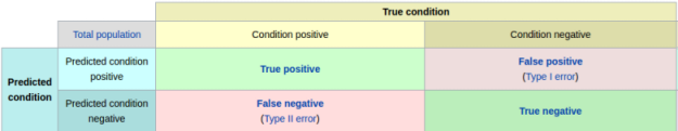
A confusion matrix compares what you predicted and the actual class labels. This creates a 2 x 2 table that quickly shows the weaknesses of your model. The language of true positives and false positives are all made clear in this table. With this table, you can create other statistics that are useful for comparing to other models.
I commonly report on these two metrics to make sure I’m being accurate with my positive classification and capturing a large part of the positive cases.
Precision: What % of your positive predictions are true positives? (True Positive / Predicted Positive)
Sensitivity / True Positive Rate: What % of the actual positives were predicted positive? (True Positive / Actually Positive)
Lift and Gains
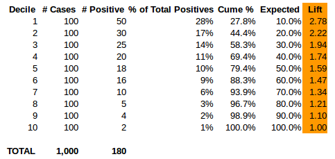
A very simple way to show the performance of your model is to create lift and gain charts. One of the best explanations of them is here. Suffice it to say, you’ll need to create a table similar to the one pictured above. It breaks down the predicted values by deciles and then calculates how many positives are captured in each decile vs the expected amount (e.g. you’d expect 10% of the positive cases to be in each decile if it were really random).
Area Under the Curve
Area Under the Curve is a very common measurement and very useful for comparing model performance. I won’t get into much details on this section but there are tools in Python and R that do this for you.
Advanced: How are the Coefficients Learned?
For those familiar with doing linear regression by hand, you’ll remember there’s some math with averages or some matrix multiplication at some point. Unfortunately, this is not the same process in logistic regression.
Instead, the coefficients are learned by iterating / changing the coefficients until the algorithm converges and finds an optimal solution. A matrix of inputs and response values are still required but to do the math directly would take way more processing power. The algorithm most commonly referred to in logistic regression is Iteratively reweighted least squares and it follows a few basic steps:
- Identify a formula / function you want to minimize (e.g. squared error).
- Calculate the derivative of that formula.
- Iteratively try coefficients and check to see if they move you closer or further from the minimization.
- Eventually, converge on a good enough answer for the coefficients.
This is why logistic regression models don’t always come out with the same coefficients. It can depend on what algorithm the software is using to find the optimal coefficients.
Bottom Line: You now have enough knowledge about logistic regression to speak intelligently about it and use it. The next thing to do is to investigate your favorite stats package and explore their many options!