Summary: Artificial Neural Networks takes input variables and multiplies them by learned weights.  The product of these numbers are then used as inputs to a “hidden” layer that acts as learned features.  The classic algorithm is called backpropogation.

Structure of a Neural Network

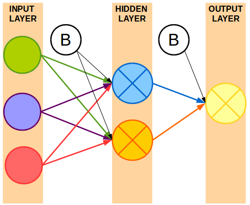
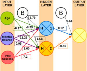
A neural network is made up of an input layer, one or more hidden layers, and an output layer.

• Input Layer: All of the input variables are represented as input nodes.
• Hidden Layer(s): All of the input variables are combined across one or more nodes in the hidden layer,
  • This essentially creates new features,derived from the inputs provided.
  • Typically all input nodes are connected to all nodes in the hidden layer.
  • If your neural network has more than one hidden layer, you’re now working with deep learning.
• Output Layer: Using the nodes in the hidden layer, a prediction or classification is made.
  • Numeric prediction uses one output node.
  • Classification uses C – 1 nodes where C is the number of classes possible.
• You’ll also notice a Bias Node for each layer.
  • A bias node acts like a regression intercept.  It’s a constant learned outside of your input data.
  • It allows you to shift the learned model.
  • Without it, any zero or negative inputs would give an output of zero.

Between these layers are connections from some or all of the nodes to nodes in the next layer. These lines represent the weight of one node into a node in the next layer. Essentially, it’s like a regression model that has coefficients that were learned and multiplied by the input value for that variable.

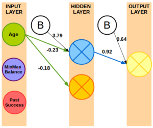
Weights produced in R using neuralnet package and Bank Marketing data set.

Using the neuralnet package in R, I created an example neural network in provided a subset of the weights above just to illustrate what some of the weights might look like.

Obligatory Biological Influence

At one point, the scientific community believed that the neurons in out brains were little dams for the electrical impulses running through our bodies. Given enough power the impulse would overcome the neuron’s threshold and fire off.

That turns out to be false but it doesn’t stop an “artificial neural network” from working so well on many data mining problems.

What Happens In the Hidden Layer(s)?

By combining all of the input variables times their weights to that node, you have the input value to the hidden layer nodes. This is just like using one model’s prediction as input to another model.

Given the combined inputs from the previous layer, the hidden nodes use an activation function to determine if the node is activated or deactivated for this row of data.

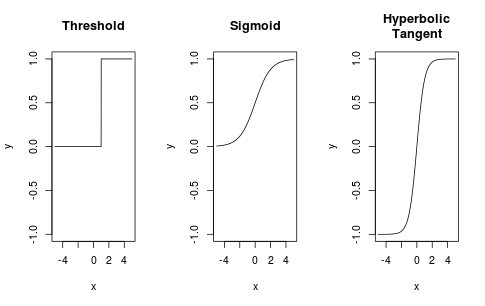
There are a few classic functions used in Neural Networks.  Each are selected because they are simple to differentiate.

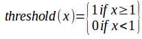
• Threshold: If the sum of all the inputs is greater than one then it outputs one. Otherwise output zero.  This is not used in modern implementations.

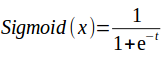
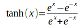
• Sigmoid: Also known as the logistic function and is the most common (or at least default) activation function used in neural networks.

• Hyperbolic Tangent: A geometric function that has a wider spread than the other two function (-1, 1) instead of (0, 1).

Each function has a maximum and minimum which is approached as you move across the x axis.  Based on the plots, you can see wider spread of hyperbolic tangent and the blunt shape of the threshold function.

After passing through the activation function, you use that node and any other nodes in the hidden layer to multiply them by their respective weights. Adding them all up creates the input to the next layer (or final output).

The activation function is only used in the hidden layer.  The output node is simply the sum of the hidden layer outputs times the weights between the hidden layer and the output layer.  Here’s an example of how data is “fed-forward” through the neural network model.

• Download Excel Example for Feed-Forward Neural Network.

The example uses trained weights seen below.

How are the Weights Learned

If you don’t know calculus, stick with this description: the weights are learned by finding the values that minimize the error by trying many different numbers as the weights. The error is used to move the weights in the right direction by moving worse performing weights faster than the rest.

If you do know calculus or are a brave soul, get ready to have some math-y fun!

Backpropogation Training Algorithm

• Select how many hidden nodes you want to use.
• Set a learning rate (small value greater than 0 and less than 1).
• Initialize random weights between each layer for every node (between -0.5 and 0.5).
• Feed the data forward:
  • Multiply input values times weights for the hidden layers.
  • Add those products together and use the sum in the activation function.
  • Take the results of the hidden layer and multiply them by weights for the output layer.
  • Add up the product for the given output node as the result for that node.
• Calculate the derivative of the error for the output layer:
  • Using the sigmoid function, the derivative is…
  • grad_out = output * (1 – output) * (actual – output)
• Calculate the derivative of the error for the hidden layer:
  • output of hidden * (1 – output of hidden) * SUM ( weights between hidden and output layers * grad_out )
• Update each network weight based on gradients:
  • new weight = current weight * learning rate * gradient * input
• Repeat the feed-forward and beyond steps until you reach some stopping condition.
  • Either a minimum error rate or a maximum number of iterations.

Did that seem complicated to you?

No?

Well then you just failed the turing test!  You must be a robot because that is complicated without working it out for yourself.  Come back soon for a step-by-step walkthrough!

There are other methods for learning the weights between nodes.  Each one offers a different approach.

Resilient Backpropogation

• Allows for undoing a step if you overshot the minimum.
• Set a maximum and minimum step size.  No learning rate or momentum.
• Faster convergence!

QuickProp

• Takes into account the previous step.
• Uses a simplified weight update formula.

Recurrent Neural Networks

• Uses a connected graph architecture to build upon previous steps.
• Used for time based or sequential data points.

Deep Learning

• Contains multiple hidden layers.

Drawbacks of Neural Networks

A neural network is an incredible tool for all sorts of machine learning applications. However, neural nets aren’t the end-all be-all.  Here are a few reasons you might want to avoid them.

Black Box: It is very difficult to interpret what is happening in a neural network. There are several papers on visualizing neural networks but mainly on image recognition and not necessarily business data sets.

Local Minima: As the algorithm works its way toward a smaller error rate, you might get caught in a local minima. You’re missing the even lower rate further away. Some algorithms incorporate a random jump to try a different section of the error curve.

Setting a Learning Rate and Hidden Node Count: Most machine learning algorithms have parameters that you have to set that controls the algorithm.  Decision trees have parent and child nodes.  K means clustering has its number of clusters.  The optimal learning rate and number of hidden nodes need to be discovered by experimentation.

Hands-On Tutorials

• Learn how to build a neural network in R.

Bottom Line: Neural Networks are robust algorithms used in many applications.  Mastering the basics, like backpropogation, allows you to step into areas like ensemble algorithms and deep learning.